As the Java 22 release is fast approaching, we took our usual look at its performance when it comes to the Timefold Solver. Read on to find out how the solver performs on Java 22, compared to Java 21. This time including GraalVM!

But first, let’s get some things out of the way.

What is Java 22 and how to get it

Java 22 is a new release of the Java platform, the trusty programming language that Timefold Solver is written in. It brings a bunch of new features, as well as the usual bugfixes and smaller improvements.

Java 22 will be generally available on March 19, 2024, but you can already try it out using the release candidate builds. We find that the easiest way to get started with Java 22 is to use SDKMAN, and that is what we did as well. We have also decided to test GraalVM for JDK 22. You may know GraalVM as the tool to run Java natively, but today we actually mean the regular JDK distribution that GraalVM provides.

While long-term support won’t likely be available for Java 22, it is still a good idea to try it out just to make sure your code is still in good shape and will be ready for the next LTS. For Timefold Solver, that means making sure the entire codebase continues to work flawlessly on Java 22, as well as running some benchmarks to ensure our users can expect at least the same performance as before. Let’s get started on that.

Micro-benchmarks

We’ll start with score director micro-benchmarks, which we use regularly to establish the impact of various changes on the performance of Constraint Streams. These benchmarks do not run the entire solver; rather, they focus exclusively on the score calculation part of the solver.

They are implemented using Java Microbenchmark Harness (JMH), and they run in many Java Virtual Machine (JVM) forks and with sufficient warmup. This gives us a good level of confidence in the results. In fact, the margin of error on these numbers is only ± 2%.

Here is the Constraint Streams performance on Java 22 vs. Java 21:

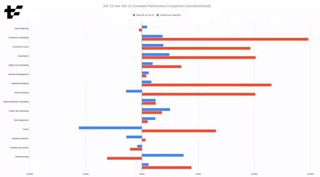
In all cases but one, the difference between OpenJDK 22 and 21 is within the margin of error for the benchmark. What that means is that we have observed no statistifically significant change in performance between the two releases. The "Tennis" benchmark is the only outlier, and it will be interesting for us to look into it and find out why.

The more interesting finding is that GraalVM for JDK 22 can be significantly faster than OpenJDK 22! With an average performance improvement of ~5% across the benchmarks, and a maximum improvement of ~15% in the "Conference Scheduling" benchmark, GraalVM is definitely worth considering for your Timefold Solver application.

It should be noted that we ran these benchmarks with ParallelGC as the garbage collector (GC), instead of the default G1GC. We are making this choice because ParallelGC has been the best GC for the solver in the past, as the solver is all about throughput and not latency.

Real-world benchmarks

Now that we’ve seen the micro-benchmarks, it’s time to compare them to real-world solver performance. This includes the entire solver, not just the score calculation part.

We ran the solver manually in 10 different JVM forks, and used the median score calculation speed. We selected a subset of the available benchmarks, to keep the run time short; the selection is representative of the entire benchmark suite in terms of heuristics used and code paths exercised. Once again, ParallelGC is used as the garbage collector. Here are the results:

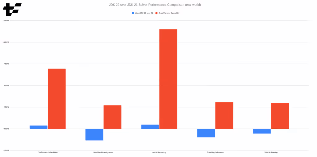
The numbers confirm the results of the micro-benchmarks. The difference between OpenJDK 22 and OpenJDK 21 is negligible, while GraalVM for JDK 22 brings improvements of up to 10 %.

Since we haven’t established a formal interval of confidence for these large benchmarks, we can’t say with certainty that the improvements are statistically significant. However, the fluctuations observed between runs have been small enough to give us confidence in the results.

Conclusion

In this post, we’ve shown that:

• Timefold Solver 1.8.0 works perfectly fine with Java 22, no changes are needed. Switching to the latest version of Java is a non-event for us here at Timefold, a testament to Java’s backward compatibility promise.
• Switching to Java 22 likely won’t bring any performance improvements or regressions for the solver.
• GraalVM for JDK 22 can bring performance improvements of up to 10 % for the solver.

Even though OpenJDK 22 doesn’t bring any performance improvements for us, we still encourage you to try Java 22. It is free after all, and you’ll be able to enjoy the latest and greatest Java platform.

Appendix A: Reproducing the results

These benchmarks use Timefold Solver 1.8.0, the latest version at the time of writing.

All benchmarks were run on Fedora Linux 39, with Intel Core i7-12700H CPU and 32 GB of RAM. We used the following JDK distributions:

• OpenJDK Runtime Environment Temurin-21.0.2+13 (21.0.2+13-LTS), available as 21.0.2-tem on SDKMAN.
• OpenJDK Runtime Environment 22.ea.36 (22+36-2370), available as 22.ea.36-open on SDKMAN.
• GraalVM for JDK 22.ea.06 (22-dev+36.1), available on Github.

Source code of the micro-benchmarks can be found in my own personal repository. The real-world benchmarks were run using timefold-solver-benchmark, using this configuration. (You’ll need timefold-solver-examples on the classpath.) Raw data used for the charts can be found in this spreadsheet.

How does your business adapt when unexpected changes disrupt your carefully planned schedules after a part of the plan has already been executed? Can you quickly adjust a vehicle routing plan when an additional urgent customer request comes in or an employee unexpectedly takes the afternoon off?

Perhaps you have read Fast Planning Optimization with the Recommended Fit API blog post by Frederico and you are wondering how to handle the cases where a new visit comes in after the route plan has started?

With Timefold, you can mark the historical part of the plan, telling the solver not to change it anymore. In addition, you can prevent changes to future parts of the plan which are to be executed "soon enough", such as redirecting a technician who had already started travelling to another customer.

In models such as Employee scheduling, marking the historical part of the plan is straightforward by using Timefold Solver’s Pinned planning entities feature. This article is focused on a more advanced pinning application for the Vehicle Routing Problem.

The Vehicle Routing Problem

The Vehicle Routing Problem (VRP) is a commonly encountered real-world scenario with numerous variants.

Let’s recall Frederico’s VRP definition from his blog post:

• The available vehicles must visit a list of locations within their capacity and before a deadline.
• The goal is to minimize the total driving time of the vehicles.

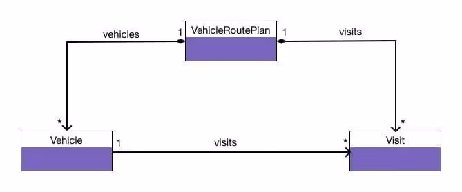
You can check the VRP quickstart and its documentation to get an idea how this scenario is implemented with Timefold.

Continuous planning example

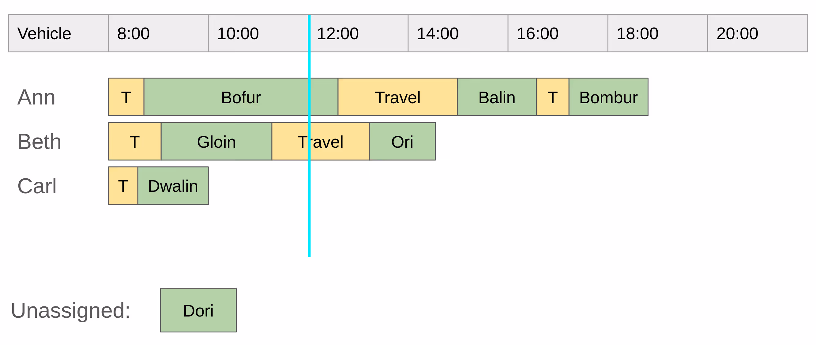
Imagine an initial plan for the day has been created and optimized before the vehicles start to work. The yellow blocks with "T" or "Travel" illustrate travelling time to the customer’s location, the green ones represent a technician’s visit at a particular customer):

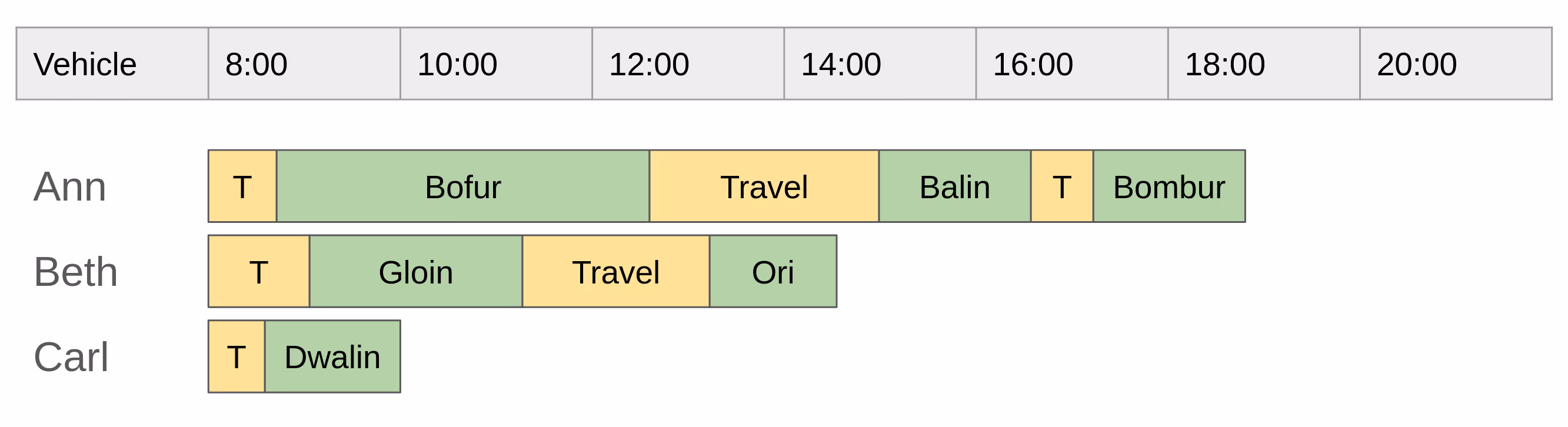
The vehicles are on their way to customers and the shift goes on as expected until noon, when a new customer calls in and needs to schedule an urgent visit for today:

The plan needs to be adjusted by including a new customer visit, but we need to let the solver know that some of the visits must not be changed (we call them pinned), either because they are already done, or a change in their planning would be disruptive. See a possible plan incorporating the change at 12:00:

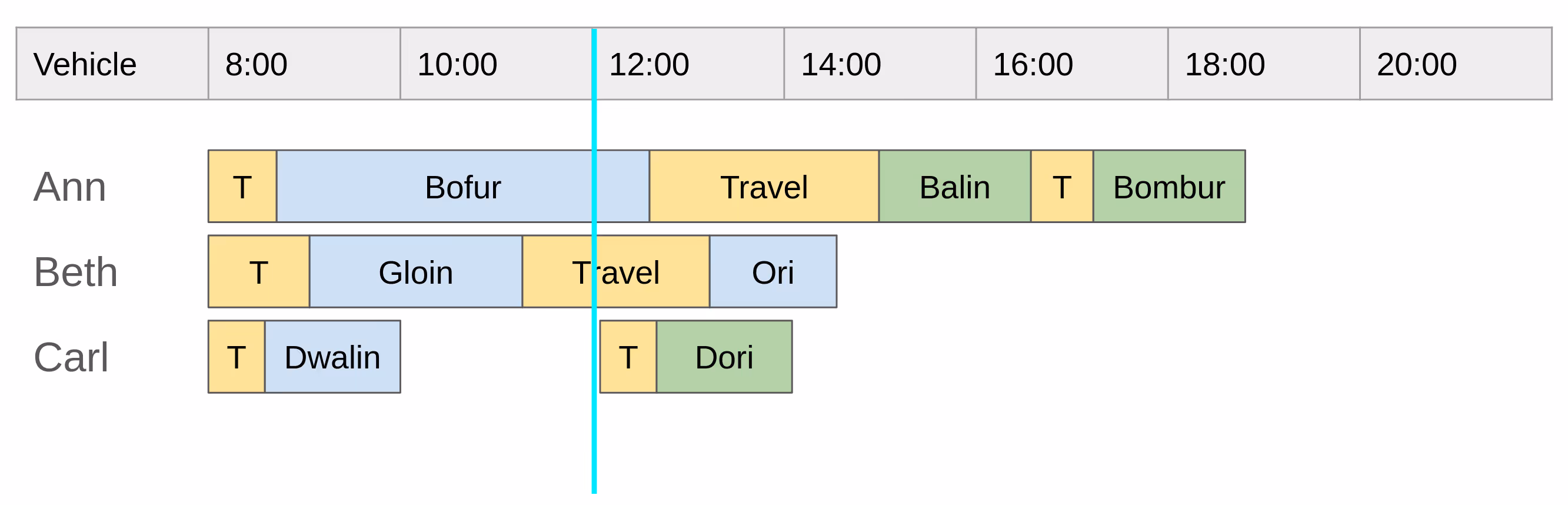
By the time of re-planning (12:00), the blue customer visits are pinned: either they have already been finished, or a vehicle has already started travelling to their location (see Beth’s last visit). Not changing their plan is the first requirement (R1) for pinning. We will discuss its implementation for VRP models shortly.

Notice the time the newly requested customer visit is planned to: travelling to the customer starts at 12:00, even though this visit has been assigned to Carl whose last visit finished around 10:00. This is the second requirement (R2) for pinning: any visit cannot be planned for a time interval already in the past. Again, we will discuss its implementation for VRP models in the next section.

The adjusted plan conforms with the above requirements and the execution continues until another customer calls in at 16:00, requesting a visit for that day:

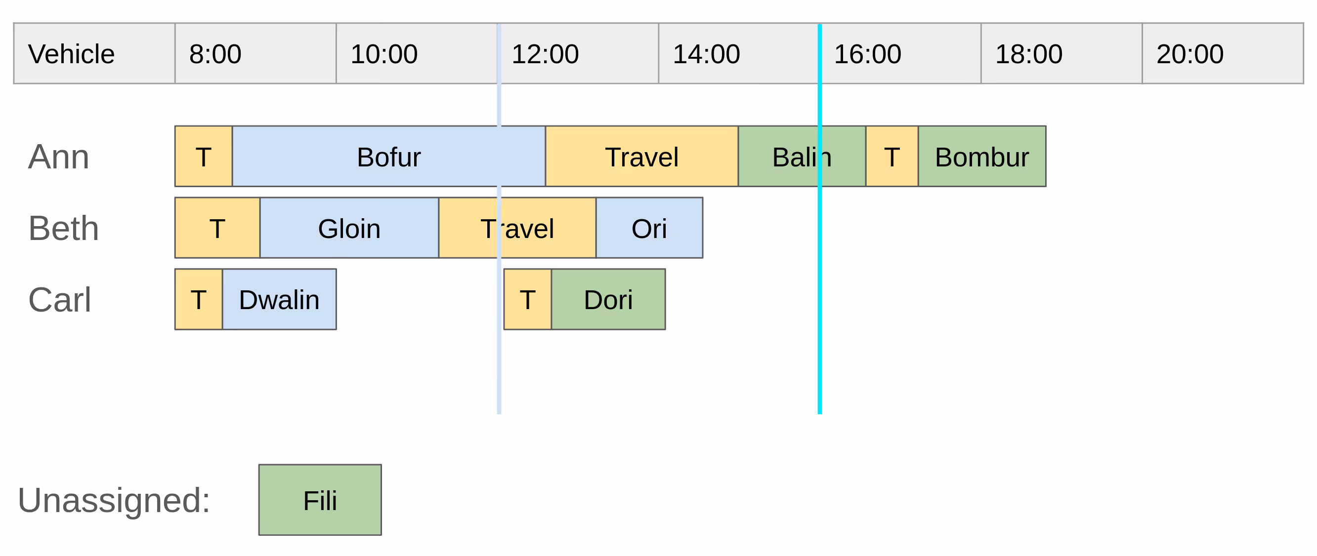
Let’s check how an updated solution at 16:00 could look like:

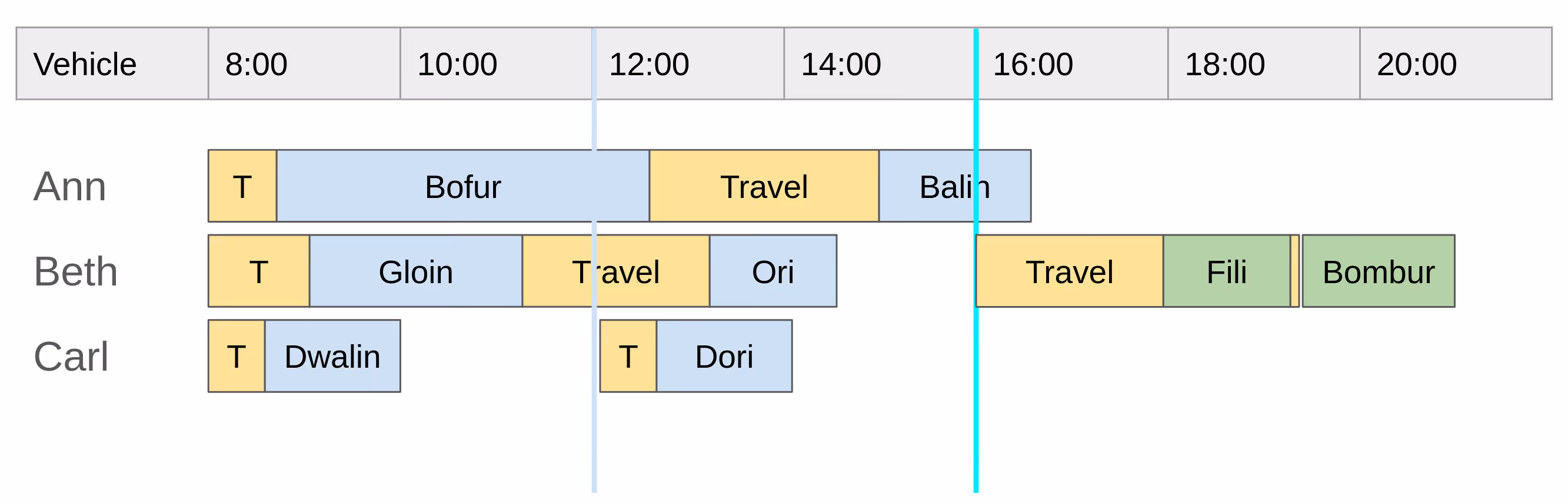
We can see that a few other visits have been finished by 16:00, therefore they were marked as pinned. The newly requested visit is planned after the time of re-planning (16:00).

In addition, you can see that the last visit originally assigned to Ann has been re-assigned to Beth. Such a re-assignment is possible, because the last visit was not pinned, and desired, because it allows the solver to find a more optimal solution: for instance by optimizing the travel distance for all vehicles as Beth’s last two visits locations are very close to each other.

Implementation

How to implement the two aforementioned requirements in a VRP model?

Requirement R1: do not change the plan for visits in history

In a VRP model, the list of visits assigned to a vehicle shift can be implemented by a Planning list variable, such as in the VRP quickstart. The requirement not to change the plan for visits that already finished can be implemented using PlanningPinToIndex, for example:

public class VehicleShift {
 // omitted other class members

 @PlanningListVariable
 private List<Visit> visits = new ArrayList<>();

 @PlanningPinToIndex
 private int firstUnpinnedIndex = 0;
}

However, we need an easy way how to specify the time instant defining which visits are to be considered pinned. For this purpose, we introduce a new attribute into the Vehicle Route Plan model, named, for instance, freezeDeparturesBeforeTime (corresponding to the blue line in the diagrams above). The model uses the attribute value to set VehicleShift.firstUnpinnedIndex (for all vehicle shifts) to the index of the first unpinned visit in the list of visits assigned to that vehicle shift.

Before submitting the plan to the solver, the model calculates the firstUnpinnedIndexvalues automatically by determining the pinned and unpinned visits using the following criteria:

• every visit ending before freezeDeparturesBeforeTime is pinned,
• every visit that a vehicle already started travelling to before freezeDeparturesBeforeTime is pinned as well,
• all other visits are unpinned.

Requirement R2: any visit cannot be scheduled for a time period in the past

By having set the VehicleShift.firstUnpinnedIndex value, we ensure that the solver can schedule any unassigned visit only after all pinned visits. However, this does not guarantee that the last pinned visit did not end several hours before freezeDeparturesBeforeTime - see Carl’s second visit in Continuous planning example.

In order to fulfil this requirement, we need to set a lower bound when a vehicle shift can start travelling to a visit and apply it during visit’s arrival time calculation in a VariableListener, based on this one from the VRP quickstart:

LocalDateTime calculateArrivalTime(Visit visit, LocalDateTime previousDepartureTime, LocalDateTime freezeDeparturesBeforeTime) {
   if (visit == null || previousDepartureTime == null) {
       return null;
   }

   LocalDateTime adjustedDepartureTime = adjustByFreezeTime(previousDepartureTime, freezeDeparturesBeforeTime);
   return adjustedDepartureTime.plusSeconds(visit.getDrivingTimeSecondsFromPreviousStandstill());
}

Let’s think about the time adjustment method implementation:

LocalDateTime adjustByFreezeTime(LocalDateTime timeToAdjust, LocalDateTime freezeDeparturesBeforeTime) {
   return freezeDeparturesBeforeTime != null && timeToAdjust.isBefore(freezeDeparturesBeforeTime) ? freezeDeparturesBeforeTime : timeToAdjust;
}

However, this approach does not work correctly when re-planning happens multiple times with different freezeDeparturesBeforeTime values - in our example scenario above, the adjustByFreezeTime(…​) method would delay the travel start of Carl’s second visit not to 12:00 but to 16:00.

To remedy the situation, we need to remember the minimum time when a vehicle is allowed to start travelling to each visit:

public class Visit {
 // other class members omitted

 private LocalDateTime minimumStartTravelTime;
}

Every unpinned visit gets the minimumStartTravelTime field set to the current value of freezeDeparturesBeforeTime, the model can do it before submitting the plan to the solver. Every pinned visit already has the value set either from the previous pinning, or, in the case of no previous pinning, the planning window start (or another sensible default):

void updateVisitsMinimumStartTravelTime(VehicleRoutePlan plan) {
   LocalDateTime effectiveMinimumStartTravelTime =
           plan.getFreezeDeparturesBeforeTime() != null ? plan.getFreezeDeparturesBeforeTime()
                   : plan.getPlanningWindow().getStartDate();

   plan.getAllVisits().forEach(visit -> {
       if (!visit.isPinned()) {
           visit.setMinimumStartTravelTime(effectiveMinimumStartTravelTime);
       } else if (visit.getMinimumStartTravelTime() == null) {
           // the edge case of freezeDeparturesBeforeTime set for the initial solving,
           // some visits may already be pinned
           visit.setMinimumStartTravelTime(plan.getPlanningWindow().getStartDate());
       }
   });
}

The adjustByFreezeTime(…​) method is adjusted to take it into account, handling multiple pinnings correctly:

LocalDateTime adjustByFreezeTime(LocalDateTime timeToAdjust, Visit visit) {
   LocalDateTime travelStartsFrom = visit.getMinimumStartTravelTime();
   return travelStartsFrom != null && timeToAdjust.isBefore(travelStartsFrom) ? travelStartsFrom : timeToAdjust;
}

Then, the arrival time calculation can look as follows:

LocalDateTime calculateArrivalTime(Visit visit, LocalDateTime previousDepartureTime) {
   if (visit == null || previousDepartureTime == null) {
       return null;
   }

   LocalDateTime adjustedDepartureTime = adjustByFreezeTime(previousDepartureTime, visit);
   return adjustedDepartureTime.plusSeconds(visit.getDrivingTimeSecondsFromPreviousStandstill());
}

Conclusion

We have shown the importance of being able to adjust a plan which already started to be executed and one possible approach to it using Pinned planning entities.

With Timefold, it is possible to handle this use-case for most models, including VRP, allowing the customer to react on unexpected requirements in time.

How does your business adapt when unexpected changes disrupt your carefully planned schedules? Can you quickly adjust a vehicle routing plan when a last-minute customer request comes in or an employee unexpectedly takes a day off? Are your current planning solutions flexible enough to handle these curveballs efficiently without requiring hours of recalibration?

The ability to swiftly respond to unforeseen circumstances isn’t just an advantage; it’s a necessity.

Timefold’s answer to this: the Recommended Fit API, providing immediate, feasible adjustments to existing plans, enabling businesses to respond to changes in real time. Whether it’s incorporating a new delivery stop or reassigning tasks due to sudden changes, the Recommended Fit API delivers quick and efficient solutions.

With Timefold, you can fetch solution recommendations and incorporate them into the final solution.

The Vehicle Routing Problem

The Vehicle Routing Problem (VRP) is a commonly encountered real-world scenario, and this article aims to use it as an example to elucidate the Recommended Fit API. It is important to understand that the Recommended Fit API is not limited to VRP, and it will work in any situation where quick responses to unexpected events are necessary.

Let’s suppose a solution for the VRP runs overnight to provide a feasible route plan for the next day. That means the process requires hours to complete. The available vehicles must visit a list of locations within their capacity and before a deadline. The goal is to minimize the total drive time of the vehicles. This article will demonstrate the feature in focus using models and resources from the VRP quickstart.

An Unexpected Phone Call

After optimizing the problem last night, the produced route plan is ready for execution. However, we receive a phone call from a customer who wishes to schedule a visit to a new location. The customer must now promptly know which vehicle to use and when to visit the new location.

We cannot re-optimize the problem with the new visit due to time constraints, as the customer is waiting on the phone. Therefore, the answer must quickly provide a feasible solution, including the new visit.

Solving Unexpected Events with the Recommended Fit API

Timefold has the Recommended Fit API that provides quicker suggestions when the problem changes. To reproduce the scenario described, please follow the steps outlined below:

1. Create an initial solution that reflects the optimization performed overnight.
2. Generate a new visit to reproduce the phone call event.
3. Call the RecommendedFit API to fetch recommendations and provide quick feedback to the client with available recommendations.
4. Once the customer chooses a recommendation, include it in the solution.

Create an Initial Solution

The Recommended Fit API expects a feasible solution as input, with all entities initialized except the one we want to add.

Generate a new location to visit

It’s worth noting that the unscheduled visit is part of the current solution visits list.Recommended Fit API searches for an uninitialized entity to start the optimization process. The process can only succeed if there is a single uninitialized entity.

Fetching recommendations with Recommended Fit API

At this moment, the customer is waiting for an answer. We need to specify three arguments to call the Recommended Fit API: the current solution, the unscheduled visit, and a proposition function that extracts the necessary details. Let’s find the visit we want to schedule:

// Find the visit
Visit visit = request.solution().getVisits().stream()
               .filter(c -> c.getId().equals(request.visitId()))
               .findFirst()
               .orElseThrow(() -> new IllegalStateException("Visit %s not found".formatted(request.visitId())));

The SolutionManager::recommendFit() function returns a list of recommendation instances. Let’s retrieve the recommendations and gather the details of the vehicles:

// Fetch the recommendations
List<RecommendedFit<VehicleRecommendation, HardSoftLongScore>> recommendedFitList =
solutionManager.recommendFit(request.solution(), visit, v -> new VehicleRecommendation(v.getVehicle().getId(), v.getVehicle().getVisits().indexOf(c)));

The recommendation call includes the current solution, unscheduled visit, and a function to extract the vehicle ID and position of the visit. As the recommendation list can be extensive, we will only provide the top five recommendations:

// Return the best five recommendations
if (!recommendedFitList.isEmpty()) {
    return recommendedFitList.subList(0, Math.min(MAX_RECOMMENDED_FIT_LIST_SIZE, recommendedFitList.size()));
}
return recommendedFitList;

The recommendation process involves evaluating the feasibility of various elements, also known as placement. Each placement receives a score based on the entire solution. The proposition function extracts the necessary information from the current placement.

After testing the placement, the solution reverts to its original state, undoing all changes made by the fitting in the placement. Therefore, the proposition function must extract data that won’t change after resetting the placement. In our example, the function extracts two pieces of information - the vehicle ID and the recommended visit position. None of them is affected or lost during the placement evaluation.

The list of recommendations sorts its elements based on their score, with the most favorable score at the top. When executing the VRP quickstart, a list of recommendations is presented as options:

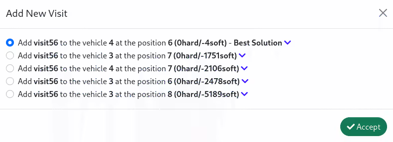
The response follows the structure of the JSON snippet provided below:

[
 {
   "proposition": {
     "vehicleId": "4",
     "index": 5
   },
   "scoreDiff": {
     "score": "0hard/-4soft",
     "constraints": [
       ...
     ]
   }
 },
 {
   "proposition": {
     "vehicleId": "3",
     "index": 6
   },
   "scoreDiff": {
     "score": "0hard/-1751soft",
     "constraints": [
       ...
     ]
   }
 }
 ...
]

Applying a Selected Recommendation

Upon receiving our recommendations, the customer selects the best one, which is the first element of the list. In order to incorporate a recommendation into a solution, let’s find the vehicle and visit targets:

// Find the target vehicle
String vehicleId = request.vehicleId();
Vehicle vehicleTarget = updatedSolution.getVehicles().stream()
           .filter(v -> v.getId().equals(vehicleId))
           .findFirst()
           .orElseThrow(() -> new IllegalStateException("Vehicle %s not found".formatted(vehicleId)));

// Find the target visit
Visit visit = request.solution().getVisits().stream()
           .filter(c -> c.getId().equals(request.visitId()))
           .findFirst()
           .orElseThrow(() -> new IllegalStateException("Visit %s not found".formatted(request.visitId())));

Next, we must insert the unscheduled visit into the designated vehicle at the specific position. Afterward, update the score of the updated solution.

// Add the visit to the target vehicle at the expected position
vehicleTarget.getVisits().add(request.index(), visit);

// Recalculate the score for the updated solution
solutionManager.update(updatedSolution);

We now have a revised route plan ready to be executed again. So far, we assumed the route plan started after the phone call. In this way, we don’t have to keep track of the routes already visited.

In cases where a new visit comes in after the route plan has started, we need to apply continuous planning techniques to manage them.

Conclusion

We explained the importance of optimization tools being able to respond quickly to unexpected events in real-life situations. Additionally, we evaluated a unique feature of Timefold Solver called Recommended Fit API, which provides feasible solutions promptly when dealing with unforeseen problem changes.

Los Angeles, 2024/02/23 - Timefold, a platform for planning optimization, built on established open-source AI solver technology, proudly announces a strategic collaboration with NGA. This partnership aims to enhance 988 Suicide & Crisis Lifeline services and streamline shift planning, ensuring prompt and effective assistance for those in need. NGA’s NEXiSLifeline solution ensures that every center has the tools required to provide life-saving assistance to all citizens.

With a network of over 200 local crisis centers and 1,000’s of call takers proficient in English and/or Spanish, efficient shift planning is imperative for the seamless operation of the 988 service. To optimize this critical aspect, Timefold has partnered with NGA. Leveraging Timefold's sophisticated employee scheduling software, NGA’s NEXiSLifeline solution ensures each center maintains optimal staffing levels, with appropriately skilled call takers available at all times.

Timefold is honored to collaborate with NGA in their mission to provide crucial support to those in need. Our optimization solutions empower centers to efficiently manage operations and deliver prompt assistance to individuals facing distress.

Maarten Vandenbroucke, CEO at Timefold

Through the integration of Timefold's cutting-edge shift planning technology, NGA remains committed to delivering around-the-clock support for those seeking help. Additionally, caller agents experience increased job satisfaction, thanks to the software's ability to consider their scheduling preferences.

The partnership between Timefold and NGA exemplifies the positive influence that optimization technology can have on critical services. Together, we stand resolute in our mission to provide immediate and effective support to individuals navigating difficult circumstances.

Don Ferguson, CEO at NGA

This collaboration marks another significant achievement for NGA, which in January forged a partnership with the state of California to introduce an innovative call-handling solution, NGA’s NEXiSLifeline across the entire state. This transformative system propels emergency communications into a digital realm, enhancing accuracy and ultimately saving valuable seconds and lives.

About Timefold Timefold is a platform for planning optimization, built on established open-source AI solver technology. It delivers advanced AI-powered optimization and scheduling technology to enhance operational efficiency. Timefold's customizable model templates empower developers to integrate cutting-edge planning models into their software. Timefold is engineered to address complex planning problems— ranging from employee scheduling and field service routing to last-mile delivery, vehicle routing and assembly line scheduling. Please visit https://timfold.ai  to learn more about the comprehensive services offered. For media inquiries and further information, please contact: Jente De Meyer, Head of Marketing, [email protected]

About NGA Next Generation Advanced: NGA is a comprehensive, adaptable, and dependable NG9-1-1 system that offers public safety emergency communication solutions that are safe and reasonably priced everywhere globally. With the most recent NG9-1-1 technology available, our gradual deployment and proprietary solutions are ready to seamlessly move traditional emergency communication systems to the future of emergency services. For more information about NEXiSLifeline and how it can transform mental health crisis response efforts, please visit https://nga911.com/nexislifeline. For media inquiries and further information, please contact:  Rebecca Dungey, Director of Marketing, [email protected].

About 988 Suicide & Crisis Lifeline The National 988 Suicide & Crisis Lifeline serves as a crucial lifeline for individuals facing emotional distress and crisis situations. Offering confidential support through calls, chats, and texts, the lifeline operates 24/7 via a network of local crisis centers and compassionate caller agents fluent in either English or Spanish. The lifeline's mission is to provide immediate assistance and promote emotional well-being for all individuals seeking help.

Do users trust your planning automation from day one? When you solve a planning problem - for example vehicle routing or maintenance scheduling - and show the optimized solution to the end-users, do they immediately like the schedule? Do they see the value in a heartbeat? Or are they extremely skeptical?

Typically, it is the latter. Because the new planning will drastically affect their lives on a daily basis: just one missing hard constraint could put them in a world of trouble.

So, how can we prove our schedule’s value? With a visualization: show the schedule in rows/columns, or on a map. But for big schedules, a visualization doesn’t show you the forest for the trees. And users really just need to verify if all constraints are taken into account.

This is where Timefold’s new ScoreAnalysis API comes into play. It explains the output of the solver AI. It breaks down the score - a mathematical concept - into business-relevant constraints. It shows you which of the trees in the forest are rotten.

Here’s an example of a ScoreAnalysis on a school timetabling schedule with a score of 0hard/-8soft:

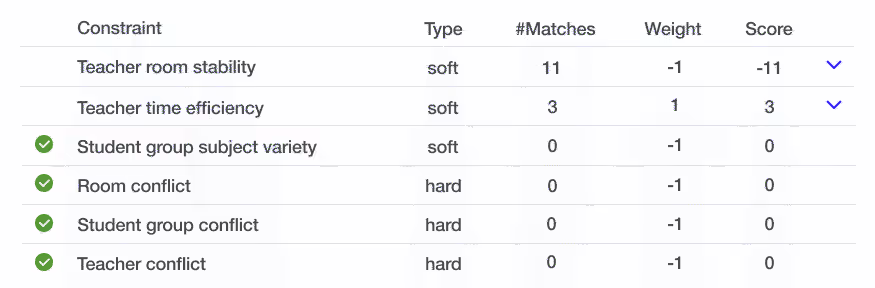
This confirms that there are no room conflicts, student group conflicts or teacher conflicts: the schedule is feasible.

It also shows 11 incidents of teachers having to switch rooms. And 3 cases of teachers benefitting from back to back lessons. The ScoreAnalysis API can even reveal when the teachers need to switch rooms, by showing the 11 matches:

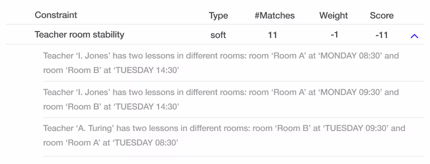
With this info, your users start to trust your automated planning.

The ScoreAnalysis API is available since Timefold Community 1.4.0. Call the SolutionManager.analyze() method to get a ScoreAnalysis instance:

var scoreAnalysis = solutionManager.analyze(solution)

This method returns quickly. Send the result to your frontend as-is: it is JSON friendly unlike our old API’s. To learn more, read our documentation or Lukas’s blog or check out the use-cases in the timefold-quickstarts repository.

Timefold AMA - vehicle routing and maintenance scheduling

When: March 19th at 08:00 PDT (San Fransisco) / 11:00 EDT (New York) / 15:00 GMT (London) / 16:00 CET (Paris/Brussels/Berlin)

Dive into the world of vehicle routing and maintenance scheduling with our Timefold Ask Me Anything (AMA) session on March 19th. This event is your chance to engage in in-depth discussions about these topics, directly with the Timefold team. Join us for an AMA with Geoffrey De Smet, creator of OptaPlanner and Co-founder of Timefold, and Lukáš Petrovický, our Timefold Solver Lead Engineer.

How to Participate

No sign-up required! On March 19th, join us on YouTube live here. Pro tip: follow our YouTube channel to get notified when we go live.

Have Questions? Let's Hear Them!

Got questions about vehicle routing, maintenance scheduling, or any other question? We'd love to hear from you in advance! Submit your questions now using this form to ensure they get prioritized during the AMA. Of course, you're also welcome to ask questions live during the event.

———

Blog

Tournament scheduling with Timefold.

2024 is an important year for soccer as it marks the 48th Copa América and the 17th EUFA EURO 2024. That made us think, can we use Timefold to create a good and fair schedule, complying with all the rules? To create this demo tournament schedule, we use Java with Quarkus.

Read the blog post

Use multiple solvers in the same application

How can you solve two different planning problems in the same application, potentially in sequence? With two SolverManager instances, one for each problem. In the article, we'll show you how to configure and inject two SolverManager instances in a single application.

Read the blog post

Timefold Solver Community Edition 1.7.0. full release notes

A feature often requested by our community is the possibility to inject more than one SolverManager in Quarkus and Spring Boot applications. We’ve heard this and 1.7.0. marks the release of it. Read more in the blog post by Frederico Gonçalves.

We're excited to see the innovative solutions you'll develop with this capability.

In addition to this we focused on bugfixes, improvements to documentation and to the quickstarts.

Here you can find all previous releases of Timefold Solver.

Latest Timefold videos

‍

What happens when a single application has to address a problem using distinct configurations? How can you solve two different planning problems in the same application, potentially in sequence? With two SolverManager instances, one for each problem. In the article, we’ll show you how to configure and inject two SolverManagerinstances in a single application.

An application may require different configurations to solve a problem or solve problem A to acquire input for solving problem B. That’s why using multiple solvers within one application becomes necessary. The Timefold Solver integrates with Quarkus and Spring Boot, making it easy to manage various solver configurations. It provides all the tools for the hassle-free configuration and utilization of distinct solvers.

In this article, we will discuss how Timefold allows us to configure multiple solver settings and explain how to use the different SolverManager instances in the application.

Distinct Solver Configurations Problem

Let’s consider a situation where we need to solve two distinct school timetabling problems:

1. Initially, a specific group of teachers is designated to teach the available lessons.
2. The next step involves assigning lessons to the rooms.

The first step will need a different domain model compared to the second. The file teachersConfig.xml shows the XML structure of the first step:

<solver xmlns="https://timefold.ai/xsd/solver" xmlns:xsi="http://www.w3.org/2001/XMLSchema-instance"
       xsi:schemaLocation="https://timefold.ai/xsd/solver https://timefold.ai/xsd/solver/solver.xsd">
 <solutionClass>org.acme.schooltimetabling.domain.TeacherToLessonSchedule</solutionClass>
 <entityClass>org.acme.schooltimetabling.domain.Teacher</entityClass>
</solver>


The following XML file, roomsConfig.xml, describes the model of the second optimization stage:

<solver xmlns="https://timefold.ai/xsd/solver" xmlns:xsi="http://www.w3.org/2001/XMLSchema-instance"
       xsi:schemaLocation="https://timefold.ai/xsd/solver https://timefold.ai/xsd/solver/solver.xsd">
 <solutionClass>org.acme.schooltimetabling.domain.Timetable</solutionClass>
 <entityClass>org.acme.schooltimetabling.domain.Lesson</entityClass>
</solver>


While we can manually create factories that instantiate managed resources for each problem, doing so requires boilerplate and error-prone code.

Injecting Multiple Instances of SolverManager

The Timefold Quarkus and Spring integrations provide built-in managed instances of the SolverManager resource for each problem definition identified during the configuration process. Therefore, there is no need for custom logic to instantiate managed resources when configuring multiple solver settings. Instead, named properties should be defined for each desired configuration. Let’s examine a simple example where we set the maximum amount of time spent on optimizing a single solver configuration in both Quarkus and Spring Boot:

Let’s add two configurations to optimize with distinct optimization time spent. One configuration runs for 5 seconds, and the other runs for 60 seconds.

We can configure multiple solvers using the namespace *.timefold.solver.<solverName> and specify the named property <solverName> for each solver. It is important to note that Quarkus configuration requires properties to have a prefixquarkus and named properties enclosed in double quotes.

Solver Configuration Properties

The following properties are supported:

[quarkus].timefold.solver.<solverName>.solver-config-xml
A classpath resource to read the solver configuration XML.

[quarkus].timefold.solver.<solverName>.environment-mode
Enable runtime assertions to detect common bugs in your implementation during development.
Defaults to REPRODUCIBLE.

[quarkus].timefold.solver.<solverName>.daemon
Enable daemon mode. Defaults to false.

[quarkus].timefold.solver.<solverName>.move-thread-count
Enable multi-threaded solving for a single problem. Defaults to NONE.

[quarkus].timefold.solver.<solverName>.domain-access-type
How Timefold Solver should access the domain model. Defaults to REFLECTION.

[quarkus].timefold.solver.<solverName>.termination.spent-limit
How long the solver can run.

[quarkus].timefold.solver.<solverName>.termination.unimproved-spent-limit
How long the solver can run without finding a new best solution after finding a new best solution.

[quarkus].timefold.solver.<solverName>.termination.best-score-limit
Terminates the solver when a specific score (or better) has been reached.


Working with Multiple Solvers

When revisiting the timetabling problem discussed in Section 2, it is necessary to fill out the properties file for both Quarkus and Spring Boot for the two distinct optimization problems in the following way:

Use the following code to inject the resources.

Conclusion

We evaluated the approach necessary to set up and use multiple solver configurations within the same application. Timefold Solver offers a simple solution for defining and utilizing different solver configurations without requiring custom logic to create and inject related managed resources.

When I started OptaPlanner 18 years ago, I couldn’t dare to imagine that one day it would schedule millions of resources. It is amazing. This would not have been possible without the dedication, innovation, and high-quality work that each core and community contributor has brought to the table.

During the Holidays, I had time to think about the past, present and future of our open source project. What did we do right? What did we do wrong? And how can we improve going forward?

In the Past, OptaPlanner evolved a lot over the years. The big leap forward started in 2020, with ConstraintStreams: constraints written in plain code. Unit test friendly. IDE friendly. Other major improvements, such as Spring/Quarkus integration and our Quickstart repository, made it easy to build REST APIs.

In the Present, we continue the OptaPlanner fork as Timefold and grow our open-source company around it. Timefold’s new score calculation engine is twice as fast, try it yourself. Our solver is now cloud friendly: lightweight (less dependencies) and fast startup times (Java native compilation), with full support for Spring Boot 3 and Quarkus 3. New features include Score Analysis to explain the score of a schedule, and Recommend Fit, to reserve a time slot for a customer on the phone.

In the Yet to Come, we will make Planning Optimization easy to use. By empowering you to develop new planning models with new constraints quickly. By making it simple to scale horizontally and integrate with map providers. We will improve the documentation, release educational videos and provision ready-to-use models. And last but not least, we will welcome Data Scientists and Operations Researchers to our open-source solver. With support for Python alongside Java and Kotlin. The future of Timefold is bright.

It’s wonderful to see how our community is growing. Join us. Together, let’s make 2024 the year of Planning Optimization!

Best regards,
Geoffrey De Smet, CTO

Releases

Timefold Solver Community Edition 1.6.0. full release notes

Featured Update - Pinning on list variables, enhancing our support for real-time planning:

Pinning of list variables
With a new @PlanningPinToIndex annotation, you can tell the solver that a certain portion of the list variable is pinned and shouldn’t be moved.

For example, for a list of customers that a vehicle will visit, this allows you to model situations where certain visits have either already happened, or where the vehicle is already too far into the trip that it would not be practical for it to turn back.

Previously, pinning was only available for the chained variable. With this, we are ramping up our efforts to bring list variable, which is easier to both understand and implement, on par with the chain variable in terms of features. Stay tuned for more on this front!

Other Enhancements:

• Solver termination can now be overridden without creating a new instance of Solver or SolverManager, look for the SolverConfigOverride class.
• The usual assortment of bugfixes and performance improvements.
• Improvements all over the documentation and quickstarts.
• Dependency upgrades.

Here you can find all previous releases of Timefold Solver

Latest Timefold videos

If you’ve ever organized a tournament with many teams, you know how hard it is to generate a good and fair tournament schedule that complies with all the rules, regardless if it’s for the national soccer league or your local padel competition.

In this article, we describe how we can create a tournament schedule and adapt it to your needs using Timefold Solver. The tournament we create is similar to a national soccer league: a fixed number of teams, each facing every other team two times.

We use Timefold Solver, which is the open-source AI solver to optimize operations and scheduling in Java, Python or Kotlin. Let’s delve deeper into the problem!

The rules of the tournament schedule

Our league consists of a variable number of teams and a variable number of rounds, with the following rules:

1. Each team has to face every other team twice, one time playing at home, the other time playing away.
2. All teams should play once per round; if the number of teams is odd, one team will not play per round.
3. The league should consist of two parts with equal rounds, with the teams switching the home stadium (eg. if the tournament has 4 rounds, round 1 and round 3 will have the same teams facing each other but the away team switching to be the home team, and vice-versa).
4. Rival teams should not face in the first round.
5. It should be prevented that the teams play many consecutive games home or away.

Let’s see how we can model that in Java with Timefold Solver.

Implementation with Timefold Solver

To create the tournament schedule, we use Java with Quarkus. The implementation is available in this GitHub repo.

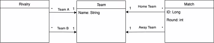
The central domain object of the problem is the team. We schedule matches that have two teams: a home team and an away team. Each match also belongs to a specific round. We also want to know the rivalries between the teams, so that we avoid having matches between rivals in the first round.

But how do we use Timefold Solver to create our schedule?

We only schedule half of the tournament, since the other half merely mirrors the rounds with the home/away teams swapped. This simplifies our scheduling problem.

Let’s suppose that we are only given the team names that are going to play in this tournament. We already know in advance the number of rounds and games per round that exist, so those are problem facts, as they don’t change during the scheduling.

Note: If the number of teams is even, the number of rounds is the number of teams minus one and the number of games per round is half of the number of teams. If the number of teams is odd, the number of rounds is the number of teams and the number of games per round is half of the number of teams minus one.

What changes during the scheduling is the teams that play in each match. So the match has the @PlanningEntity annotation and the home team and the away team have the @PlanningVariable annotation. The solver changes the @PlanningVariables in the @PlanningEntity annotated objects to optimize the solution. More information about problem facts and planning entities can be seen in the docs.

@PlanningEntity
public class Match {

   @PlanningId
   private Long id;

   @PlanningVariable
   private Team homeTeam;

   @PlanningVariable
   private Team awayTeam;

   private int round;

   public Match() {
   }

   public Match(Long id, int round) {
       this.id = id;
       this.round = round;
   }

   public Long getId() {
       return id;
   }
   public Team getHomeTeam() {
       return homeTeam;
   }

   public Team getAwayTeam() {
       return awayTeam;
   }

   public int getRound() {
       return round;
   }
}

We also need a class that is our @PlanningSolution, with the problem facts for the problem. Let’s call it TournamentSchedule.

This object has a list of teams from which the solver can choose to populate the schedule. That is indicated by the annotation @ValueRangeProvider.

It is also needed to annotate with @ProblemFactCollectionProperty the problem facts to be used by the constraints, as well as the list of matches to optimize, with@PlanningEntityCollectionProperty.

@PlanningSolution
public class TournamentSchedule {

   @PlanningEntityCollectionProperty
   private List<Match> matches;

   @ValueRangeProvider
   @ProblemFactCollectionProperty
   private List<Team> teams;

   @ProblemFactCollectionProperty
   private List<Rivalry> rivalries;

   @PlanningScore
   private HardSoftScore score;

   public TournamentSchedule() {
   }

   public TournamentSchedule(List<Team> teams, List<Rivalry> rivalries) {
       this.matches = generateMatches(teams);
       this.teams = teams;
       this.rivalries = rivalries;
   }

   private List<Match> generateMatches(List<Team> teams) {
       int numberOfRounds = (teams.size() % 2 == 0) ? teams.size() - 1 : teams.size();
       int gamesPerRound =  teams.size() / 2;
       List<Match> matches = new ArrayList<>();
       int id = 0;
       for(int round: IntStream.range(0, numberOfRounds).boxed().toList()) {
           for(int game: IntStream.range(0, gamesPerRound).boxed().toList()) {
               matches.add(new Match((long) id++, round));
           }
       }
       return matches;
   }

   public List<Match> getMatches() {
       return matches;
   }

   public List<Rivalry> getRivalries() {
       return rivalries;
   }

   public HardSoftScore getScore() {
       return score;
   }

   @Override
   public String toString() {
       StringBuilder result = new StringBuilder();
       matches.stream().collect(Collectors.groupingBy(Match::getRound))
               .forEach((round, matches) -> {
           result.append("Round ").append(round).append(": \n");
           String roundMatchesString = matches.stream()
                   .map(match -> "\t" + match.getHomeTeam().getName() + " vs " + match.getAwayTeam().getName())
                   .collect(Collectors.joining("\n"));
           result.append(roundMatchesString).append("\n\n");
       });
       return result.toString();
   }
}

Now that our entities are set up, let’s create an empty list of constraints.

public class ScheduleConstraintProvider implements ConstraintProvider {
   @Override
   public Constraint[] defineConstraints(ConstraintFactory constraintFactory) {
       return new Constraint[] {};
   }
}

Finally, let’s create an endpoint, and create four teams with two rivalries, so that we can run the solver!

@Path("/solve")
public class SolverResource {

   @Inject
   SolverManager<TournamentSchedule, UUID> solverManager;

   @GET
   public String solve() {
       UUID problemId = UUID.randomUUID();
       List<Team> teams = List.of(
               new Team("A"),
               new Team("B"),
               new Team("C"),
               new Team("D")
       );

       List<Rivalry> rivalries = List.of(
               new Rivalry(teams.get(0), teams.get(1)),
               new Rivalry(teams.get(0), teams.get(2))
       );

       TournamentSchedule problem = new TournamentSchedule(teams, rivalries);
       // Submit the problem to start solving
       SolverJob<TournamentSchedule, UUID> solverJob = solverManager.solve(problemId, problem);
       TournamentSchedule solution;
       try {
           // Wait until the solving ends
           solution = solverJob.getFinalBestSolution();
       } catch (InterruptedException | ExecutionException e) {
           throw new IllegalStateException("Solving failed.", e);
       }
       return solution.toString();
   }

}

Start the application and try it out!

> mvn quarkus:dev❯ curl localhost:8080/solve
Round 0:
A vs A
A vs A

Round 1:
A vs A
A vs A

Round 2:
A vs A
A vs A

It seems that the first team is chosen to play in all rounds! That happened because we do not have any constraints yet. There is nothing to tell the solver which situations it should prefer or avoid. Let’s add them!

Constraints

Let’s start with the basic constraints and see where our schedule looks funny. The first thing we don’t want is that a team is scheduled to play against itself.

In Timefold Solver, we can configure hard and soft constraints. A hard constraint cannot be broken, and breaking a hard constraint would mean that the solution is not acceptable. Soft constraints can be broken but that should be avoided. Since a team playing against itself is impossible, let’s configure it as a hard constraint. More information about constraints and score is available in the docs.

   @Override
   public Constraint[] defineConstraints(ConstraintFactory constraintFactory) {
       return new Constraint[] {
               teamCannotPlayAgainstItself(constraintFactory),
       };
   }


   private Constraint teamCannotPlayAgainstItself(ConstraintFactory constraintFactory) {
       return constraintFactory
               .forEach(Match.class)
               .filter(match -> match.getHomeTeam() == match.getAwayTeam())
               .penalize(HardSoftScore.ONE_HARD)
               .asConstraint("A team cannot play against itself");
   }❯ curl localhost:8080/solve
Round 0:
B vs A
B vs A

Round 1:
B vs A
B vs A

Round 2:
B vs A
B vs A

Great! By running the solver, we see that now no team is facing itself, but there are always the same two teams facing each other. Let’s add a hard constraint so each two teams can only face once (Rule 1).

   @Override
   public Constraint[] defineConstraints(ConstraintFactory constraintFactory) {
       return new Constraint[] {
               teamCannotPlayAgainstItself(constraintFactory),
               twoTeamsCanOnlyFaceOneTime(constraintFactory)
       };
   }

   //...

   private Constraint twoTeamsCanOnlyFaceOneTime(ConstraintFactory constraintFactory) {
       return constraintFactory
               .forEachUniquePair(Match.class)
               .filter((match1, match2) -> (match1.getHomeTeam() == match2.getHomeTeam() &&
                       match1.getAwayTeam() == match2.getAwayTeam()) ||
                       (match1.getHomeTeam() == match2.getAwayTeam() &&
                               match1.getAwayTeam() == match2.getHomeTeam())
               )
               .penalize(HardSoftScore.ONE_HARD)
               .asConstraint("Two teams can only face each other one time");
   }❯ curl localhost:8080/solve
Round 0:
B vs A
C vs A

Round 1:
D vs A
C vs B

Round 2:
D vs B
D vs C

Now teams are only facing each other once, but are still playing more than once per round (see the A team in the first round) (Rule 2). Let’s add another hard constraint to solve that.

   @Override
   public Constraint[] defineConstraints(ConstraintFactory constraintFactory) {
       return new Constraint[] {
               teamCannotPlayAgainstItself(constraintFactory),
               twoTeamsCanOnlyFaceOneTime(constraintFactory),
               teamOnlyOnceInRound(constraintFactory)
       };
   }

   // ...

   private Constraint teamOnlyOnceInRound(ConstraintFactory constraintFactory) {
       return constraintFactory
               .forEachUniquePair(Match.class, equal(Match::getRound))
               .filter((match1, match2) -> match1.getHomeTeam() == match2.getHomeTeam()
                       || match1.getAwayTeam() == match2.getHomeTeam()
                       || match1.getHomeTeam() == match2.getAwayTeam()
                       || match1.getAwayTeam() == match2.getAwayTeam()
               )
               .penalize(HardSoftScore.ONE_HARD)
               .asConstraint("Each team can only play once per round");
   }❯ curl localhost:8080/solve
Round 0:
B vs A
D vs C

Round 1:
C vs A
D vs B

Round 2:
D vs A
C vs B

Wow, now the schedule is starting to look much more feasible. No more physical impossibilities neither impossible rounds. We are just breaking two more rules. Teams are playing too many consecutive games at home or away (Rule 5). For example, team D is always playing at home. Let’s implement a soft constraint to avoid that.

   @Override
   public Constraint[] defineConstraints(ConstraintFactory constraintFactory) {
       return new Constraint[] {
               teamCannotPlayAgainstItself(constraintFactory),
               twoTeamsCanOnlyFaceOneTime(constraintFactory),
               teamOnlyOnceInRound(constraintFactory),
               // Soft constraints
               eachTeamShouldNotPlayManyConsecutiveGamesAtHomeOrAway(constraintFactory)
       };
   }

   // ...

   private Constraint eachTeamShouldNotPlayManyConsecutiveGamesAtHomeOrAway(ConstraintFactory constraintFactory) {
       return constraintFactory
               .forEachUniquePair(Match.class)
               .filter(
                       (match1, match2) -> (match1.getRound() == match2.getRound() + 1 &&
                               (match1.getHomeTeam() == match2.getHomeTeam() || match1.getAwayTeam() == match2.getAwayTeam())) ||
                               (match1.getRound() + 1 == match2.getRound() &&
                                       (match1.getHomeTeam() == match2.getHomeTeam() || match1.getAwayTeam() == match2.getAwayTeam()))
               )
               .penalize(HardSoftScore.ONE_SOFT)
               .asConstraint("A team should not play two consecutive house or away games");
   }❯ curl localhost:8080/solve
Round 0:
B vs A
D vs C

Round 1:
C vs B
A vs D

Round 2:
C vs A
D vs B

We can see that sometimes it’s impossible for all teams to not play two consecutive away and home matches (for example, D is playing rounds 1 and 2 away), but we can limit that to at most once per team. Finally, the rival teams are A with B and A with C. So we would like to start the schedule with the game A vs D. Let’s implement another soft constraint to avoid rival teams facing each other in the first round (Rule 4).

   @Override
   public Constraint[] defineConstraints(ConstraintFactory constraintFactory) {
       return new Constraint[] {
               teamCannotPlayAgainstItself(constraintFactory),
               twoTeamsCanOnlyFaceOneTime(constraintFactory),
               teamOnlyOnceInRound(constraintFactory),
               // Soft constraints
               eachTeamShouldNotPlayManyConsecutiveGamesAtHomeOrAway(constraintFactory),
               rivalTeamsShouldNotFaceOnFirstRound(constraintFactory)
       };
   }

   // ...

   private Constraint rivalTeamsShouldNotFaceOnFirstRound(ConstraintFactory constraintFactory) {
       return constraintFactory
               .forEach(Match.class)
               .filter(match -> match.getRound() == 0)
               .join(Rivalry.class)
               .filter((match, rivalry) ->
                       (match.getHomeTeam() == rivalry.getTeamA() && match.getAwayTeam() == rivalry.getTeamB()) ||
                               (match.getHomeTeam() == rivalry.getTeamB() && match.getAwayTeam() == rivalry.getTeamA())
               )
               .penalize(HardSoftScore.ONE_SOFT)
               .asConstraint("Rival teams should not face on first round");
   }❯ curl localhost:8080/solve
Round 0:
D vs A
C vs B

Round 1:
A vs C
B vs D

Round 2:
B vs A
D vs C

Now we have a full tournament scheduling algorithm according to the rules. The best part is that now it is possible to create a tournament with as many teams as we want to. For example, you can see the full scheduling for 20 teams and no rivalries below.

❯ curl localhost:8080/solve
Round 0:
N vs K
L vs C
R vs D
S vs B
J vs I
E vs Q
H vs T
F vs A
G vs O
P vs M

Round 1:
L vs H
S vs Q
O vs M
A vs C
J vs E
I vs T
G vs F
C vs R
N vs P
D vs K

Round 2:
S vs D
A vs J
L vs E
H vs P
G vs B
N vs C
L vs T
F vs O
I vs Q
R vs M

Round 3:
I vs S
E vs D
N vs G
B vs C
J vs H
O vs A
M vs Q
F vs K
R vs T
P vs L

Round 4:
T vs F
H vs Q
I vs L
C vs K
E vs M
J vs N
D vs O
I vs B
S vs P
G vs R

Round 5:
E vs T
F vs D
Q vs B
G vs S
A vs P
I vs N
B vs R
L vs K
C vs H
O vs J

Round 6:
Q vs K
D vs I
S vs N
M vs R
G vs L
P vs B
H vs O
E vs F
N vs T
C vs J

Round 7:
G vs E
I vs K
O vs O
C vs F
B vs H
R vs N
S vs A
J vs P
T vs D
M vs L

Round 8:
K vs S
L vs R
I vs G
H vs F
M vs B
J vs T
A vs Q
E vs P
M vs N
D vs C

Round 9:
K vs H
S vs L
M vs J
G vs D
T vs C
I vs I
P vs O
B vs E
A vs H
R vs Q

Round 10:
P vs R
I vs O
D vs A
L vs N
M vs S
F vs J
H vs G
E vs K
T vs B
C vs Q

Round 11:
N vs S
T vs M
R vs I
A vs L
J vs D
P vs F
H vs H
O vs K
E vs S
G vs Q

Round 12:
C vs R
N vs H
M vs G
K vs T
J vs B
I vs F
L vs D
P vs Q
A vs E
O vs S

Round 13:
E vs C
I vs A
R vs O
D vs Q
K vs B
S vs T
G vs P
F vs N
H vs M
L vs J

Round 14:
I vs P
E vs N
H vs R
K vs K
T vs O
C vs G
J vs S
Q vs L
A vs B
M vs D

Round 15:
C vs P
O vs Q
T vs L
K vs M
C vs I
G vs A
B vs N
J vs R
E vs H
S vs F

Round 16:
I vs M
L vs B
O vs C
Q vs F
P vs T
A vs K
H vs D
O vs N
R vs S
G vs E

Round 17:
F vs L
K vs J
T vs Q
T vs G
R vs A
P vs D
S vs H
C vs M
O vs B
E vs I

Round 18:
A vs T
N vs Q
C vs S
E vs R
L vs O
F vs M
J vs G
B vs D
K vs P
I vs H

We suggest you to add your own rules to try the solver, such as:

• Add a list of referees to the problem and try to attribute them to each match fairly: each of them should have a similar number of matches, with no more than one match per round, and a similar number of matches between the teams.
• Schedule the matches between closer teams to earlier in the tournament.
• Take into account the time and schedule the matches between rivals to the peak hours with no match overlapping another.

Share your experiments with the community. We can’t wait to know what you build!

In the past, you’ve worked with OptaPlanner. This globally used Open Source software was at the core of a wide array of planning optimization projects, significantly impacting efficiency in diverse industries. My co-founder, Geoffrey De Smet, the creator of OptaPlanner, and I witnessed first-hand the transformative impact of this technology. Driven by our mission to Free the world from wasteful scheduling we decided to build upon this legacy. Thus, Timefold was born.

As announced on May 2nd, 2023, OptaPlanner continues as Timefold. When the future of OptaPlanner at Red Hat seemed uncertain, we took the initiative to ensure that this vital technology not only survives but also thrives. Timefold represents not merely a stable continuation but also an evolution - a new chapter. We already fixed a good number of bugs and released new features. Timefold is twice as fast, and comes with better documentation. But this is just the start as our ambition reaches far higher into making our planning optimization products as accessible and easy to use as database technology or even spreadsheets!

We are honored to welcome the core OptaPlanner team - Lukas, Radovan, and Christopher - to Timefold. Their expertise and insights are invaluable in our journey ahead. We are proud of the Timefold team and thankful for being on this ride together.

Timefold is more than a tool; it’s a community and a movement. Your contributions, feedback, and ideas are the keystones of this community. Find us on StackOverflow or star us on GitHub.

We invite you to continue on this journey with us. We will send out a monthly newsletter that we will keep informative and on-point. Feedback is always welcome. We look forward to your continued support and engagement!

Why upgrade OptaPlanner to Timefold?

For reliability, features and speed. Timefold adds features and fixes bugs, many that still reside in OptaPlanner. Timefold is twice as fast as OptaPlanner out-of-the-box. Here’s how to upgrade OptaPlanner to Timefold.

Releases

Timefold Solver Community Edition 1.5.0 full release notes

Featured Update: Recommended Fit API, designed for appointment scheduling. Whilst on a call, operators can receive a list of appointment choices, ranked from best fit to worst, for informed decision-making. Also, score corruption errors now provide better debugging information.

Timefold Solver Community Edition 1.4.0 full release notes

Featured Update: JSON-friendly score explanations. Timefold Solver can now break down the score all the way to individual constraint matches. It can also compute differences between any two solutions. Also, Spring Boot integration has improved significantly.

Here you can find all previous releases of Timefold Solver.

Latest Timefold videos

What the team likes about Timefold Solver:

Coding the capacitated VRP in Java:

Geoffrey De Smet & Lukáš Petrovický at Devoxx Belgium:

‍