Performance is a top priority for Timefold Solver, since any performance gains means we can find the same solution in a less amount of time (or alternatively, a better solution in the same amount of time). This is also true for Python, which is typically one or two orders of magnitudes slower than Java. Through a variety of techniques, we are able to make Python reach 25% of Java’s throughput. Read on to find out the methods we deploy to make Python’s performance better, and see how Timefold Solver for Python performance compares to Java on a variety of PlanningAI models.

Note: Usage of Python in this article refers exclusively to the CPython implementation.

Why is Python relatively slow?

Python’s performance challenges are mostly due to design decisions:

Global Interpreter Lock

The Global Interpreter Lock, or GIL for short, is a lock that prevents multiple threads from executing Python code at the same time. This is because Python’s core data structures, such as dict, list and object are not thread-safe.

When the GIL was introduced (Python 1.5, in the year 1998), multi-threaded programs were rare (most computers only supported one thread at the time), and as such, using a GIL simplifies Python extension developer experience and does not degrade single-threaded perfrmance. The GIL was a good idea for its time, but gradually became worse as multi-threaded programs and computers became more common. Currently, Python s working on removing the GIL, but it will be several releases before it is widely available.

Dynamically Typed

Python is dynamically typed, which means the result type of operations cannot be determined before their execution. Moreover, many operations such as addition and attribute lookup are also dynamic, since they look up attributes on their operands' types. As a result, this seemly simple python code:

def add(x, y):
   return x + y

Does something a lot more complex underneath:

def ignore_type_error_if_builtin_type(arg_type, method, x, y):
   try:
      return method(x, y)
   except TypeError:
       if arg_type in [int, str, list, ...]:
           return NotImplemented
       raise

def add(x, y):
   x_type = type(x)
   x_add = x_type.__dict__.get('__add__')
   y_type = type(y)
   y_radd = y_type.__dict__.get('__radd__')
   if x_add is None and y_radd is None:
       raise TypeError('...')
   elif y_radd is None:
       out = ignore_type_error_if_builtin_type(x_type, x_add, x, y)
       if out is NotImplemented:
           raise TypeError('...')
       return out
   elif x_add is None:
       out = ignore_type_error_if_builtin_type(y_type, y_radd, y, x)
       if out is NotImplemented:
           raise TypeError('...')
       return out
   else:
       if x_type != y_type and issubclass(y_type, x_type):
           out = ignore_type_error_if_builtin_type(y_type, y_radd, y, x)
           if out is NotImplemented:
               out = ignore_type_error_if_builtin_type(x_type, x_add, x, y)
               if out is NotImplemented:
                   raise TypeError('...')
       else:
           out = ignore_type_error_if_builtin_type(x_type, x_add, x, y)
           if out is NotImplemented:
               out = ignore_type_error_if_builtin_type(y_type, y_radd, y, x)
               if out is NotImplemented:
                   raise TypeError('...')
       return out

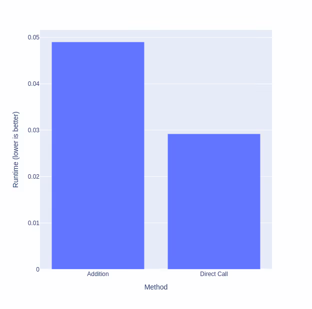
For custom types, this complexity causes addition to have about double the overhead of a direct method call:

import timeit

source = \
'''
class A:
   def __init__(self, value):
       self.value = value

   def __add__(self, other):
       return self.value + other.value

a = A(0)
b = A(1)
'''
timeit.timeit('a + b', source)
#  0.04903000299964333

timeit.timeit('add(a, b)', f'{source}\nadd=A.__add__')
#  0.029219600999567774

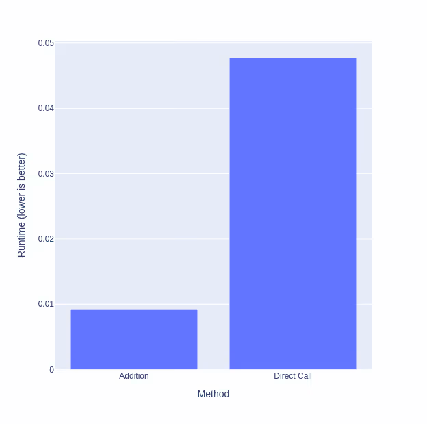
However, Python specializing adaptive interpreter speeds up the code for builtin types, such as int.

import timeit

timeit.timeit('a + b', 'a=0\nb=1')
#  0.009246169998732512

timeit.timeit('add(a, b)', 'a=0\nb=1\nadd=int.__add__')
#  0.04777865600044606

Monkey-Patching

Python supports monkey-patching; that is, the behavior of types and functions can be modified at runtime. For example, you can change the implementation of a type’s method:

class Dog:
   def talk(self):
       return 'Woof'

a = Dog()
print(a.talk())  # Prints 'Woof'

Dog.talk = lambda self: 'Meow'
print(a.talk())  # Prints 'Meow'

Monkey-patching prevents method inlining, an optimization technique where a method is copied into its call sites, removing call overhead and allowing further optimization to be done.

Lack of a JIT compiler

Python currently lacks a JIT compiler, meaning it cannot optimize code based on runtime characteristics (such as how often a branch is taken). This will probably change in the future, as a experimental JIT compiler for Python is currently being worked on.

However, all the above is insignificant to what was our biggest performance obstacle…​

Proxies are slow

A proxy is a class that acts as a facade for arbitrary classes. In order for Java to call a Python method (or vice versa), a Foreign Function Interface must be used. A Foreign Function Interface, or FFI in short, is an interface that allows one program language to call functions of another. In Java, there are currently two different FFI implementations:

• Java Native Interface (JNI)
• (Java 22 and above) Foreign Function and Memory API (foreign)

JNI and the foreign API both returns a raw pointer (in JNI, a long, and in foreign, a MemorySegment) for Python objects. However, a pointer has little use in Java code, which expects interfaces like Comparable or Function. Typically, proxies are used to convert the pointer into Comparable, Function, or some other interface.

Why Proxies are slow

If a proxy is empty, it is only about 1.63 slower than a direct call. However, proxies are often not empty. Often, they need to do complex tasks such as converting the arguments and results of methods. How slow are we talking? Consider this simplistic benchmark:

public class Benchmark {
   public static void benchmark(Runnable runner) {
       var start = System.nanoTime();
       for (int i = 0; i < 10_000; i++) {
          runner.run();
       }
       var end = System.nanoTime();
       System.out.printf("%.9f\n", (end - start) / 1_000_000_000d);
   }

   public static void main(String[] args) {
       System.out.println("Cold");
       benchmark(() -> {});

       System.out.println("Hot");
       benchmark(() -> {});

   }
}

Which we can invoke via JPype

import jpype

jpype.startJVM(classpath=['.'])
benchmark = jpype.JClass('Benchmark')

@jpype.JImplements('java.lang.Runnable')
class Runner:
   @jpype.JOverride
   def run(self):
       pass

print("Cold")
benchmark.benchmark(Runner())

print("Hot")
benchmark.benchmark(Runner())

or GraalPy:

import java.Benchmark

def run():
   pass

print("Cold")
java.Benchmark.benchmark(run)

print("Hot")
java.Benchmark.benchmark(run)

Here are the runtimes for running benchmark with an empty Runnable in Java versus an empty Runnable implemented as a Python proxy:

MethodRuntimeJava Direct Call (Cold)0.000232610Java Direct Call (Hot)0.000240525Java FFI Direct Call (Cold)0.005904000Java FFI Direct Call (Hot)0.000442477JPype Proxy (Cold)0.006906666JPype Proxy (Hot)0.004721682GraalPy Proxy (Cold)0.027417475GraalPy Proxy (Hot)0.000883732

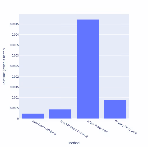
Despite the Python code literally doing nothing, a JPype proxy is 967.102% slower than a direct Python call when hot. GraalPy fares better at only 100% slower than a direct Python call. Things get even worse when there are arguments and return types involved (for example, with java.util.function.Predicate). Here, we pass a Python list to Java (which calls a Python proxy function on each item in a list).

import jpype

jpype.startJVM(classpath=['.'])
benchmark = jpype.JClass('Benchmark')


class Item:
   def __init__(self, value):
       self.value = value


@jpype.JImplements('java.util.function.Predicate')
class Runner:
   @jpype.JOverride
   def test(self, item):
       return item.value


def proxy(item):
   return jpype.JProxy(jpype.JClass('java.io.Serializable'), inst=item, convert=True)


arraylist = jpype.JClass('java.util.ArrayList')
items = arraylist([proxy(Item(i % 2 == 0)) for i in range(10000)])

print('Cold')
benchmark.benchmark(Runner(), items)

print('Hot')
benchmark.benchmark(Runner(), items)

or GraalPy:

import java.Benchmark


class Item:
   def __init__(self, value):
       self.value = value


def test(item):
   return item.value


items = [Item(i % 2 == 0) for i in range(10000)]
print("Cold")
java.Benchmark.benchmark(test, items)

print("Hot")
java.Benchmark.benchmark(test, items)

MethodRuntimeJava Direct Call (Cold)0.000819039Java Direct Call (Hot)0.000559228Java FFI Direct Call (Cold)0.004265137Java FFI Direct Call (Hot)0.000807377JPype Proxy (Cold)0.015507570JPype Proxy (Hot)0.012130092GraalPy Proxy (Cold)0.070494332GraalPy Proxy (Hot)0.004472111

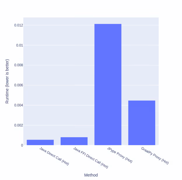
Here, JPype is 1402.41% slower than calling Python directly when hot! GraalPy also degraded, becoming 453.906% slower than calling Python directly.

In particular, when the arguments are passed to Java, they are converted to Java proxies. However, when the arguments are passed back to Python, they are not converted back to Python objects. Instead, a Python proxy is created for the Java proxy, creating additional overhead for every single operation.

Why using FFI directly is hard

Given the problems with proxies, the obvious solution is to just manage the opaque Python pointers and do direct Python calls. Unfortunately, using FFI directly is hard:

• In order for garbage collection to work, the Java and Python garbage collectors must be aware of each other (especially if Java objects are passed to Python). In particular, if an arena is closed, it is zeroed out (to prevent use-after-free). This means if Python is still tracking the object (because it retains a reference), a segmentation fault will occur on the next garbage collection. However, if an arena is never closed, we will eventually run out of memory. This is especially true for long running processes, such as solving. JPype solves this with deep magic that links Java’s and Python’s garbage collectors. Unfortunately, calling Python functions directly using FFI is unsupported in JPype.
• Java FFI is designed around starting from Java, not from Python (i.e. Java host). As a result, without doing deep magic like JPype, a separate Java process must be launched to use FFI with an independent Python interpreter.
• Java objects cannot be used as Python objects directly, meaning some proxies will need to be generated if a Java object is passed to Python code.

Avoiding all the problems (and replacing them with new ones)

So how can we avoid the performance losses from:

• Global Interpreter Lock
• Dynamically Typed Code
• Monkey Patching Support
• No JIT Compiler
• Proxy Overhead

with a single solution? The (not so simple) answer is to translate Python’s bytecode and objects to Java bytecode and objects.

• No Global Interpreter Lock, as Java doesn’t have one.
• Can treat type annotations as strict, meaning we can determine which method to call at compile time in some cases.
• Can remove monkey patching support; by the time the code is compiled, typically all monkey patching (if any) is already done.
• Java has a JIT compiler.
• Because the Python objects are translated to Java objects, no proxies are involved.

However, there is a not so simple part:

• Unlike Java, Python’s bytecode changes drastically from version to version. Even the behavior of existing opcodes may change (i.e. Python bytecode is neither forwards nor backwards compatible).
• Python’s bytecode has several quirks that makes it non-trivial to directly map it to Java bytecode. For instance, Python keeps its for loop’s iterator on the stack for the entire for loop body. As a result, when an exception is caught in a for loop, Python bytecode expects there to still be an iterator on the stack (whereas in Java, the exception handler’s stack is always empty).
• The Java object result needs to be converted back to a Python object.

Annoying as these problems are, they are significantly easier to debug and test than using FFI directly; we can rely on JPype’s deep magic to keep Java’s and Python’s garbage collectors in sync, and we can have deterministic reproducers and test cases.

How the translated bytecode performance?

Is it truly worth all the hassle of translating Python’s bytecode? Well, the only way to know is to measure the speed before and after the bytecode translation. Bytecode translation was originally implemented in OptaPy (which Timefold Solver for Python is a fork of), which included an option to use the proxies instead. Since the bytecode generation became more mature, the option to use proxies was removed from Timefold Solver for Python.

Thus, to compare the performance of proxies versus translated bytecode, we will use the latest (and probably last) release OptaPy (9.37.0b0) on Python 3.10.

Here are the score calculation speeds of using proxies versus translated bytecode in OptaPy’s school timetabling quickstart (higher is better).

Note: OptaPy’s School Timetabling quickstart is not equivalent to Timefold’s School Timetabling quickstart: there are bugs in the constraints that are fixed in the Timefold versions but were never addressed in OptaPy’s version.

MethodScore Calculation SpeedProxies599/secTranslated Bytecode69558/sec

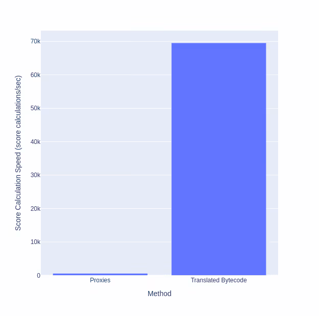
In short, using translated bytecode multiplied our throughput by 100 (i.e. an over 100,000% performance increase)!

So…​ how fast is Timefold Solver for Python?

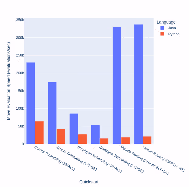
Now finally to the topic of the blog post: how fast is Timefold Solver for Python on various PlanningAI models? Below are the move evaluation speeds of the Java and Python Timefold 1.15.0 quickstarts:

QuickstartDatasetLanguageMove Evaluation SpeedSchool TimetablingSMALLJava 22.0.1230143/secSchool TimetablingSMALLPython 3.1264034/secSchool TimetablingLARGEJava 22.0.1174881/secSchool TimetablingLARGEPython 3.1242249/secEmployee SchedulingSMALLJava 22.0.185926/secEmployee SchedulingSMALLPython 3.1227462/secEmployee SchedulingLARGEJava 22.0.153265/secEmployee SchedulingLARGEPython 3.1215753/secVehicle RoutingPHILADELPHIAJava 22.0.1330492/secVehicle RoutingPHILADELPHIAPython 3.1218912/secVehicle RoutingHARTFORTJava 22.0.1337094/secVehicle RoutingHARTFORTPython 3.1221443/sec

In short:

• School Timetabling in Python is about 75% slower than Java
• Employee Scheduling in Python is about 70% slower than Java
• Vehicle Routing in Python is about 95% slower than Java

Where is performance lost?

If the Python bytecode is translated to Java bytecode, why is it still significantly slower than Java? There are several differences between the translated bytecode and normal Java bytecode:

• The translated bytecode must be consistent with Python’s semantics. This means:
  • Cannot use 32-bit int or 64-bit long to represent a Python’s int, since Python’s int are BigInteger.
  • Although some dynamic dispatches during operations such as addition can be determined statically, others cannot either due to missing or lost type information. In Java, all dispatches are determined at compile time.
  • In the case a function expects a Java return type or argument, a conversion to the appropriate Java/Translated Python type must occur.
• The translated bytecode is far from idiomatic Java bytecode. As such, the Java JIT compiler, designed for idiomatic Java bytecode, might have trouble optimizing it. Even Fernflower (a Java decompiler) has trouble decompiling the translated bytecode!
• Inlining opportunities are limited, due to the generated bytecode’s size and usage of interfaces.

What does the result mean in practice?

• For school timetabling and employee scheduling, to get the same result as Java in Python, you should run it about four times longer duration, (so if Java runs for 1 minutes, Python should run for 4 minutes).
• For vehicle routing, to get the same result as Java in Python, you should run it about twenty times longer duration, (so if Java runs for 1 minutes, Python should run for 20 minutes).

In many cases, this performance loss is acceptable, as it allows you to write your code in pure Python instead of Java, meaning:

• No requirement to learn Java.
• No requirement to make a separate Java model that matches your Python model.
• Can use Python libraries like Pydantic, FastAPI and Pandas to create the planning problem and to process solutions.

Note: Python libraries might use functions defined in C, which naturally have no corresponding Python bytecode, and thus cannot be translated to Java bytecode.

Usage of C‑defined functions in constraints causes a necessary fallback to Python, and the Java objects need to be converted back to Python objects. This causes a massively performance degradation that has roughly the same performance as proxies.

C‑defined functions can be used outside of constraints without issue.

Conclusion

To make Timefold’s goal of making PlanningAI accessible to everyone a reality, everyone should be able to write in the language of their choice. For many, that language is Python.

To make writing PlanningAI models in Python practical, the Python solver must match a reasonable fraction of the Java Solver’s performance. This is a challenge, as Python provides a myriad of obstacles to performance. But like any obstacle, they can be overcome.

By overcoming these obstacles, we managed to make the Python solver match 25% of the Java solver’s performance, making writing PlanningAI models in Python practical. That being said, for use cases that truly require the most performant code, it is probably best to stick to Java.

Timefold, a Belgian AI software startup specializing in planning optimization, has successfully raised €6 million in a seed funding round led by Lakestar, one of Europe’s top venture capital firms. Returning investor Smartfin also participated in the round. This funding will accelerate the development and commercialization of Timefold’s groundbreaking PlanningAI technology, designed to optimize complex scheduling and routing challenges faced by large-scale enterprises.

The round follows a €2 million pre-seed funding secured in March 2023, led by Smartfin, which fueled the initial development and market introduction of Timefold's platform. The company’s software, based on the open-source OptaPlanner project, aims to solve inefficiencies in large-scale planning for industries such as logistics, transportation, field services, and workforce management.

Timefold’s platform is already trusted by several Fortune 500 companies, including Deutsche Bahn, Palantir, NEC, ADP, and Advantage Solutions. The new funding will enable Timefold to further scale its offerings, focusing on building out its platform and further developing planningAI models for other mission-critical applications.

A Game-Changing Solution for Scheduling Problems

Timefold’s PlanningAI platform is poised to eliminate the inefficiencies caused by inadequate planning solutions. Many businesses today face a choice between lengthy development cycles with custom-built models or underpowered off-the-shelf tools. Timefold offers a more powerful alternative—enterprise-ready models that can be easily integrated via REST APIs, reducing the need for expensive consultancy retainers or in-house expertise.

Geoffrey De Smet, CTO and co-founder of Timefold, highlighted the company’s vision:
"Planning is everywhere and often hidden in plain sight, yet efficient schedules are rare. From the field service technician coming to fix your boiler, to the plane assigned to your next flight: schedules run the world. We are tackling complex planning problems by providing out-of-the-box planning models for IT teams to run, test, and configure easily. It is easy to use, no math, and no need for consultants. Our API plugs seamlessly into your software, and with Lakestar’s backing, we can help businesses deploy planning that increases productivity, improves employee happiness, and reduces carbon emissions."

Proven Success and Growing Demand

Timefold is already making a significant impact across multiple industries. Companies like Palantir Technologies have partnered with Timefold to integrate their advanced scheduling optimizers across their Foundry platform.

"Palantir has collaborated with the Timefold team to make their world-class scheduling optimisers available across our Foundry and AI Platforms. The team’s experience, the depth of their solutions, and their willingness to dive into hard problems has enabled us to deliver significant outcomes for our customers. We are excited about their fundraise and look forward to scaling our impact together into the future,"

Molly Carmody, Planning Optimisation Lead at Palantir

Backed by Industry Leaders

"Geoffrey's life's work has been to revolutionize how complex NP-hard problems are addressed, saving enterprises, governments, and infrastructure providers hundreds of millions of euros annually. For 18 years, his leading open-source technology has optimized critical operations, scheduling shifts for thousands of police officers, routing millions of parcels, assigning gates at major airports, and planning national train timetables."

When we met Geoffrey, Maarten, and the rest of the Timefold team, we recognized how uniquely talented this team is and the outsized potential of a category winner in the making. ‍

Enrico Mellis, principal at Lakestar

Mellis added:

"Maarten brings vital entrepreneurial expertise to propel Geoffrey’s vision to market. The solution's unmatched maturity and clear product-market fit, bolstered by partnerships with giants like Palantir, promise to transform operations across multiple industries."

Leadership and Growth

Timefold’s executive team includes industry veterans who have joined from top software companies like Showpad, Tinder, Qualtrics, and Techwolf, further strengthening its position to drive innovation and growth. CEO and co-founder Maarten Vandenbroucke commented:

"Typically, companies are left with two extreme choices: build their own models which take long development cycles and costly consultancy retainers, or use underpowered automation tools. With Timefold, neither is necessary. We have enterprise-ready models for field service routing, employee scheduling, production planning, and more in development. Our clients are already achieving better outcomes and faster time-to-market, which significantly reduces risk from their end."

Imagine reducing your code by 90% while making your optimization models more efficient and easier to maintain. Sounds impossible? Not anymore. With Timefold’s new @CascadingUpdateShadowVariable, you can streamline complex planning tasks—like updating the arrival times in a vehicle route—into just a few lines of code. In this article, I’ll show you how this powerful new feature can simplify your codebase, enhance performance, and free you from the tedious task of writing custom listeners. We will demonstrate how to simplify the Vehicle Route Problem (VRP), turning 60 lines of code into 5.

Timefold Solver has a useful feature called shadow variables. A shadow variable is a planning variable that can be deduced from the state of genuine planning variables, such as the arrival time of a given visit or the following visit of a vehicle route. The shadow variable @ShadowVariable provides an approach that allows implementing a custom listener to update the variable values.

Before Timefold Solver 1.13.0, you would update a chain of connected elements using the @ShadowVariable listener. This robust solution can be applied to any related use case. However, at Timefold, we aim to simplify your life by offering solutions that enhance your models' understandability and improve their performance. And now we’ve made it so that creating a separate listener to update source variables is sometimes unnecessary.

The upcoming sections will initially discuss the requirements for updating the tail chains. Following that, the different approaches for configuring a listener that updates a specified source shadow variable and triggers changes to the subsequent elements of a planning list variable will be explained.

Tail chains need updating

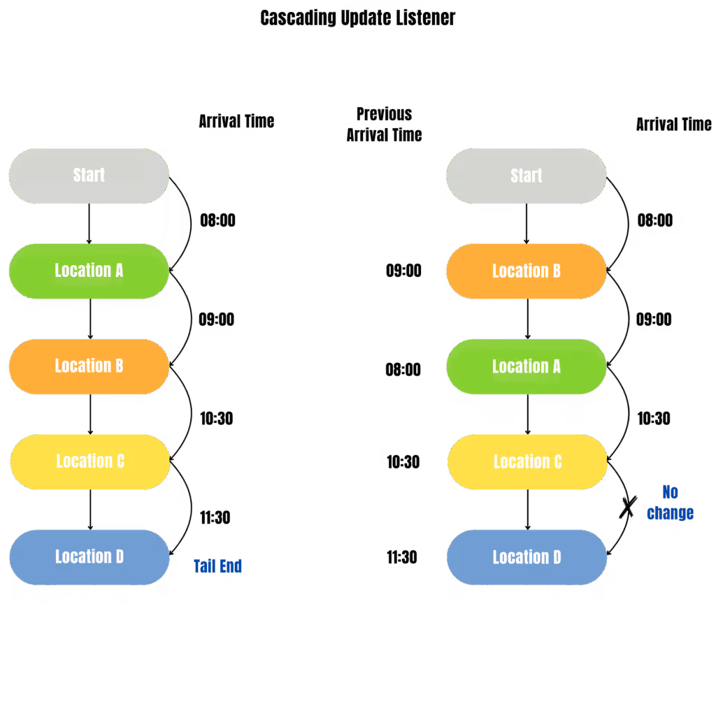
Let’s consider the VRP problem definition. Given a set of vehicles and a list of locations to visit, each visit carries the expected arrival time to the destination. We estimate the arrival time based on the arrival time to the previous location and the travel time between locations.

In the previous image, the vehicle arrives at Location A at 08:00. After that, it travels to Location B, arriving at 09:00, and then travels to Location C. We have a series of related locations that need to be updated sequentially. That means if there are any changes in the arrival time at Location A, all subsequent locations must update their arrival times. In other words, a tail chain update is needed.

To illustrate the use case, let’s take a look at the Visit model class:

public class Visit {
   ...
   @InverseRelationShadowVariable(sourceVariableName = "visits")
   private Vehicle vehicle;
   @PreviousElementShadowVariable(sourceVariableName = "visits")
   private Visit previousVisit;
   @NextElementShadowVariable(sourceVariableName = "visits")
   private Visit nextVisit;
   ...
   private LocalDateTime arrivalTime;
}

The arrivalTime field contains the vehicle’s arrival time, which the constraint can utilize to impose penalties for missing deadlines. The next two sections explain how to use the @ShadowVariable and @CascadingUpdateShadowVariable listeners, respectively.

The old way: implementing shadow variable listeners

The @ShadowVariable triggers a listener when one or more source shadow variables change. Let’s update the model Visit:

public class Visit {
   ...
   @InverseRelationShadowVariable(sourceVariableName = "visits")
   private Vehicle vehicle;
   @PreviousElementShadowVariable(sourceVariableName = "visits")
   private Visit previousVisit;
   @NextElementShadowVariable(sourceVariableName = "visits")
   private Visit nextVisit;
   @ShadowVariable(variableListenerClass = ArrivalTimeUpdatingVariableListener.class, sourceVariableName = "vehicle")
   @ShadowVariable(variableListenerClass = ArrivalTimeUpdatingVariableListener.class, sourceVariableName = "previousVisit")
   private LocalDateTime arrivalTime;
}

Next, let’s implement the ArrivalTimeUpdatingVariableListener:

public class ArrivalTimeUpdatingVariableListener
   implements VariableListener<VehicleRoutePlan, Visit> {
   ...
   @Override
   public void afterVariableChanged(ScoreDirector<VehicleRoutePlan> scoreDirector, Visit visit) {
       if (visit.getVehicle() == null) {
           if (visit.getArrivalTime() != null) {
               scoreDirector.beforeVariableChanged(visit, ARRIVAL_TIME_FIELD);
               visit.setArrivalTime(null);
               scoreDirector.afterVariableChanged(visit, ARRIVAL_TIME_FIELD);
           }
           return;
       }
       Visit previousVisit = visit.getPreviousVisit();
       LocalDateTime departureTime =
               previousVisit == null ? visit.getVehicle().getDepartureTime() : previousVisit.getDepartureTime();
       Visit nextVisit = visit;
       LocalDateTime arrivalTime = calculateArrivalTime(nextVisit, departureTime);
       while (nextVisit != null && !Objects.equals(nextVisit.getArrivalTime(), arrivalTime)) {
           scoreDirector.beforeVariableChanged(nextVisit, ARRIVAL_TIME_FIELD);
           nextVisit.setArrivalTime(arrivalTime);
           scoreDirector.afterVariableChanged(nextVisit, ARRIVAL_TIME_FIELD);
           departureTime = nextVisit.getDepartureTime();
           nextVisit = nextVisit.getNextVisit();
           arrivalTime = calculateArrivalTime(nextVisit, departureTime);
       }
   }
   ...
}

Whenever the vehicle or previousVisit changes, the listener automatically updates the subsequent visits.

The new way: simplifying with Cascading Updates

As of Timefold Solver 1.13.0, the @CascadingUpdateShadowVariable does not require a separate listener class. Instead, we add a new method to the domain class that updates the related shadow variables. Let’s update the Visit class with the cascading shadow variable annotation:

public class Visit {
   ...
   @InverseRelationShadowVariable(sourceVariableName = "visits")
   private Vehicle vehicle;
   @PreviousElementShadowVariable(sourceVariableName = "visits")
   private Visit previousVisit;
   @NextElementShadowVariable(sourceVariableName = "visits")
   private Visit nextVisit;
   @CascadingUpdateShadowVariable(targetMethodName = "updateArrivalTime")
   private LocalDateTime arrivalTime;
}

After that, we need to add a method called updateArrivalTime with the logic to update arrivalTime:

private void updateArrivalTime() {
   if (previousVisit == null && vehicle == null) {
       arrivalTime = null;
       return;
   }
   LocalDateTime departureTime = previousVisit == null ? vehicle.getDepartureTime() : previousVisit.getDepartureTime();
   arrivalTime = departureTime != null ? departureTime.plusSeconds(getDrivingTimeSecondsFromPreviousStandstill()) : null;
}

The method must not be static and must not accept any parameters. Timefold Solver triggers updateArrivalTime after all events are processed. Therefore, the listener will be the last one executed during the event lifecycle. Additionally, it automatically propagates changes to the subsequent visits and stops when the arrivalTime value does not change or when it reaches the end.

Conclusion

Updating a set of interconnected elements in a specific order is a common scenario when defining your optimization model. Timefold Solver provides different solutions for defining listeners that update shadow variable sources in a specific sequence. The new Cascading Update Shadow Variable simplifies creating listeners for planning list variables, resulting in code that is easier to write, read, and maintain.

Load balancing is a common constraint for many Timefold use cases. Especially when scheduling employees, the workload needs to be spread out fairly. For example, nurses in your hospital care that everyone works the same number of weekends, and there may even be legal requirements to that effect. Join us as we show you how to bring fairness to your Timefold solution.

Defining fairness

Fairness is a complex concept, and it is not always clear what is fair. For example, let’s assign 15 undesirable tasks to five employees. Each task takes a day, but the tasks have different skill requirements. In a perfectly fair schedule, each employee will get three tasks, because the average is 15 / 5 = 3. Unfortunately, this doesn’t solve the entire problem, because there are other constraints. For example, there are seven tasks that require a skill which only two of the employees possess. One of them will have to do at least four tasks.

From the above, we can see that our schedule cannot be perfectly fair, but we can make it as fair as possible. We can define fairness in two opposing ways:

• A schedule is fair if most users think it is fair to them.
• A schedule is fair if the employee with the most tasks has as few tasks as possible.

Since we want to treat all employees equally, the second definition is correct. Besides, if we make almost everyone happy by letting one employee do all the work, that employee would probably quit, and that doesn’t help.

Let’s look at a few different solutions of the same dataset, sorted from most to least fair. Each one has 15 tasks:

AnnBethCarlDanEdSolution QualitySchedule A33333Most fairSchedule B44322 Schedule C53322 Schedule D55221 Schedule E63321 Schedule F56211 Schedule G150000Most unfair

Ann has the most tasks each time. How do we compare schedules in which Ann has the same number of tasks?

AnnBethCarlDanEdSolution QualitySchedule C53322Schedule D55221

We look at the second most loaded employee, Beth. In schedule D, she has five tasks, while in schedule C, she has less. This makes schedule C fairer overall. Therefore, this is the definition of fairness we use in the remainder of this post.

Measuring unfairness

For the mathematically minded among you, we’re currently using the following formula to calculate the unfairness of a solution, also called "squared deviation from the mean":

In this formula:

• n is the number of employees.
• xi is the number of tasks assigned to employee i.
• x̄ is the average number of tasks per employee.

Also see a MathExchange question discussing this formula and other alternatives in depth.

Implementing fairness constraints

Timefold Solver supports fairness constraints out of the box through the use of grouping and the load-balancing constraint collector. In your ConstraintProviderimplementation, a load-balancing constraint may look like this:

Java

Constraint balanceEmployeeShiftAssignments(ConstraintFactory constraintFactory) {
   return constraintFactory.forEach(Shift.class)
           .groupBy(ConstraintCollectors.loadBalance(Shift::getEmployee))
           .penalizeBigDecimal(HardSoftBigDecimalScore.ONE_SOFT, LoadBalance::unfairness)
           .asConstraint("Balance employee shift assignments");
}

Kotlin

fun balanceEmployeeShiftAssignments(constraintFactory: ConstraintFactory): Constraint {
   return constraintFactory.forEach(Shift::class.java)
       .groupBy(ConstraintCollectors.loadBalance({ shift -> shift.employee }))
       .penalizeBigDecimal(HardSoftBigDecimalScore.ONE_SOFT) { loadBalance -> loadBalance.unfairness }
       .asConstraint("Balance employee shift assignments")
}

Python

def balance_employee_shift_assignments(constraint_factory: ConstraintFactory):
   return (constraint_factory.for_each(Shift)
           .group_by(ConstraintCollectors.load_balance(lambda shift: shift.employee))
           .penalize_decimal(HardSoftDecimalScore.ONE_SOFT, lambda load_balance: load_balance.unfairness())
           .as_constraint("Balance employee shift assignments")
           )

This constraint will penalize the solution based on its unfairness, defined in this case by how many ShiftAssignment are allocated to any particular Employee.

Unfairness is a dimensionless number that measures how fair the solution is. A lower value indicates a fairer solution. The smallest possible value is 0, indicating that the solution is perfectly fair. There is no upper limit to the value, and it is expected to scale linearly with the size of your dataset. The value is rounded to six decimal places.

Different unfairness values may only be compared for solutions coming from the same dataset. Unfairness values computed from different datasets are incomparable.

Important: When using fairness constraints, we recommend that you use one of the score types based on BigDecimal, such as HardSoftBigDecimalScore. See Timefold documentation for a detailed rationale.

Conclusion

Fairness in your planning improves employee satisfaction and helps you comply with legal requirements. Adding fairness to your Timefold solution is straightforward and can be done in a few lines of Java, Python or Kotlin code. Other solvers would be hard-pressed to match the flexibility of our implementation. Check out the latest Timefold Solver and start making your solutions fairer today.

In Python, data scientists have a rich, open source AI toolkit to handle any business challenge, except for planning and scheduling. How do you optimally route field service technicians, assign employees to shifts, or schedule maintenance jobs?

For large organizations, solver technologies can reduce operational costs by $100,000,000 and CO² emissions by 10 million kg. So why doesn’t every Data Scientist use optimization solvers?

It’s because solvers are notoriously hard to use. Even a simple Vehicle Routing Problem implementation involves dealing with mathematical equations. Most solvers are too complex to handle real-world complexity. That’s about to change.

We are excited to announce Timefold Solver for Python, the new open source solver for Python developers and data scientists. It’s easy to use, powerful, and fast.

Solve a planning problem by calling solve():

solution = solver.solve(problem)

Timefold is built for real-world complexity, such as Field Service Routing, Maintenance Scheduling, Employee Scheduling, Last Mile Delivery, and Task Assignment. It’s not optimized for a simple Traveling Salesman Problem. It scales to large datasets with business constraints for tens of thousands of employees, and more.

Timefold Solver for Python is free to use (open source under the Apache License),documented, thoroughly tested, and released on PyPi. It’s backed by our open core company that lives and breathes planning optimization.

Just pip install timefold and run one of the quickstarts:

Hello worldEmployee SchedulingVehicle Routing ProblemSchool Timetabling

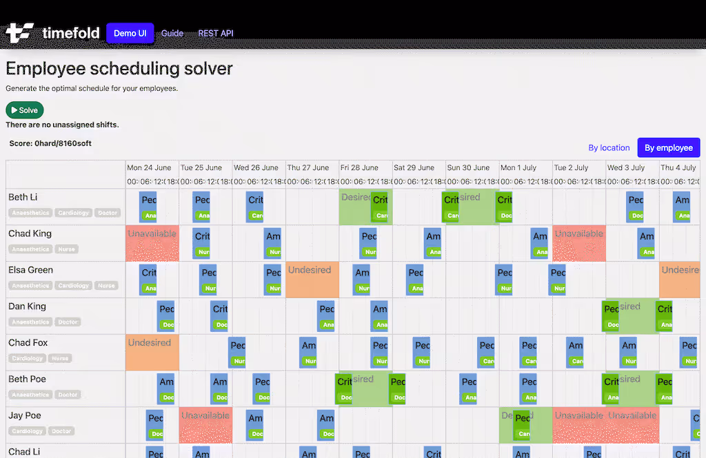
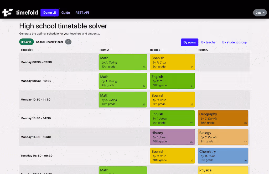
Each quickstart comes with a fully functional REST API, unit tests, and web UI.

Easy to use

Timefold puts developer productivity front and center. In Timefold, you define your model as domain classes and your constraints as code.

No need for mathematical equations. No need for a double array of binary variables. Timefold is the solver for Data Scientists and Software Engineers, not mathematicians. It integrates naturally with the rest of your Python software stack.

Let’s take a look at the source code for Employee Scheduling and Vehicle Routing:

Employee Scheduling

In Employee Scheduling, assign shifts to employees, while adhering to labor regulations and employee availability requests. It’s commonly used for healthcare personnel, security guards, police, or any employees that work in shifts.

Domain code

The Employee class has the name and skills of an employee:

class Employee:
   name: str
   skills: set[str]

The Shift class contains the start and end of each shift, as well as the required skill.

It also has an employee field, annotated with PlanningVariable. That’s the field(s) that Timefold changes during solving. Because it contains such an annotated field, the class has a @planning_entity decorator.

@planning_entity
class Shift:
   start: datetime
   end: datetime
   required_skill: str
   employee: Annotated[Employee | None, PlanningVariable]

Employee and Shift are custom domain classes, so you can add attributes as needed, for your constraints, to fulfill your business requirements.

Constraints

Timefold assigns each shift to an employee, taking into account the constraints, such as:

• Required skill: Every assigned employee must have the required skill. Add this as a hard constraint:

# For each shift ...
(constraint_factory.for_each(Shift)
 # ... that is assigned an employee that doesn't have the required skill ...
 .filter(lambda shift: shift.required_skill not in shift.employee.skills)
 # ... penalize as an infeasible solution
 .penalize(HardSoftScore.ONE_HARD)
 .as_constraint("Missing required skill"))

• Ten hours between shifts: Ideally, an employee has 10 hours between two shifts. Add this as a soft constraint (AKA an objective):

# For each shift ...
(constraint_factory.for_each(Shift)
 # ... combined with a later shift with the same employee ...
 .join(Shift,
   Joiners.equal(lambda shift: shift.employee.name),
   Joiners.less_than_or_equal(lambda shift: shift.end, lambda shift: shift.start)
 )
 # ... with less than 10 hours in between ...
 .filter(lambda first_shift, second_shift:
       (second_shift.start - first_shift.end).total_seconds() // (60 * 60) < 10)
 # ... penalize as a soft constraint weighted by the number of minutes less than 10 hours
 .penalize(HardSoftScore.ofSoft(1), lambda first_shift, second_shift:
       600 - ((second_shift.start - first_shift.end).total_seconds() // 60))
 .as_constraint("At least 10 hours between 2 shifts"))

• Fairness: All employees are assigned the same amount of work.
• and many more

Each constraint is unit tested. Run pytest on a quickstart to validate every constraint works as you intended:

def test_required_skill():
   ann = Employee(name="Ann", skills={"Doctor"})
   (constraint_verifier.verify_that(required_skill)
   .given(ann,
          Shift(start=..., end=..., required_skill="Nurse", employee=ann))
   .penalizes(1))
   beth = Employee(name="Beth", skills={"Nurse"})
   (constraint_verifier.verify_that(required_skill)
   .given(beth,
          Shift(start=..., end=..., required_skill="Nurse", employee=beth))
   .penalizes(0))

Vehicle Routing

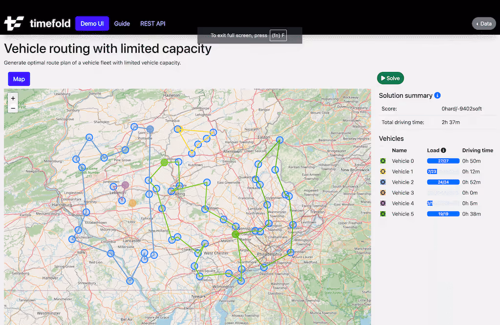
In the Vehicle Routing Problem, assign each visit to a vehicle and decide the order of the visits for each vehicle. The goal is to minimize driving time while adhering to capacity, time windows, overtime, and other constraints.

Domain

The Vehicle class has a list of visits, annotated with PlanningListVariable. Timefold fills in the list of visits:

@planning_entity
class Vehicle:
   name: str
   home_location: Location
   visits: Annotated[list[Visit], PlanningListVariable]
   ... # shift hours, capacity, skills, ...

The Visit class has a name and location:

class Visit:
   name: str
   location: Location
   ... # time windows, weight/volume usage, skill requirements, ...

Constraints

Constraints, such as the capacity constraint, are written in code:

def vehicle_capacity(factory: ConstraintFactory):
   return (factory.for_each(Vehicle)
           .filter(lambda vehicle: vehicle.calculate_total_demand() > vehicle.capacity)
           .penalize(HardSoftScore.ONE_HARD,
                     lambda vehicle: vehicle.calculate_total_demand() - vehicle.capacity)
           .as_constraint("Vehicle capacity"))

This approach has the following benefits:

Powerful

Many solvers claim to be the fastest solver. But even the fastest solver is useless if it can’t implement all of your business requirements:

• Hard constraints are physical or legal limitations. For example, an employee can’t be in two places at the same time.
• Medium constraints assign as much work as possible, without breaking hard constraints. Ideally, all work is assignable, but on some days there is more work than people to do it.
• Soft constraints (AKA objectives) reduce costs, increase service quality, and improve employee retention. For example, minimize traveling time or minimize overtime. These constraints are aggregated into a weighted function.

If a solution breaks a single hard constraint, the entire solution is useless. But also, every soft constraint that is missing constitutes a hidden cost to the company.

Therefore, Timefold can handle any constraint. Not just linear constraints. Not just quadratic constraints. Even constraints such as fairness and load balancing are fully supported.

Reliable, fast, and scalable

Timefold is built for complex business constraints and large datasets. It uses significantly less memory than traditional solvers, allowing it to scale beyond traditional limitations.

Because of many internal performance optimizations, it’s extremely fast. Even with custom code in your constraints. Under the hood, it uses a JVM to speed up performance.

To orchestrate high-scale datasets or maps integration, Timefold is developing a proprietary Enterprise extension.

Get Started

Timefold Solver for Python is ready to automate and optimize your operations scheduling challenges.

Get started with one of the quickstarts today:

$ git clone https://github.com/TimefoldAI/timefold-quickstarts.git
...
$ cd timefold-quickstarts/python/hello-world
...
$ pip install -e .
...
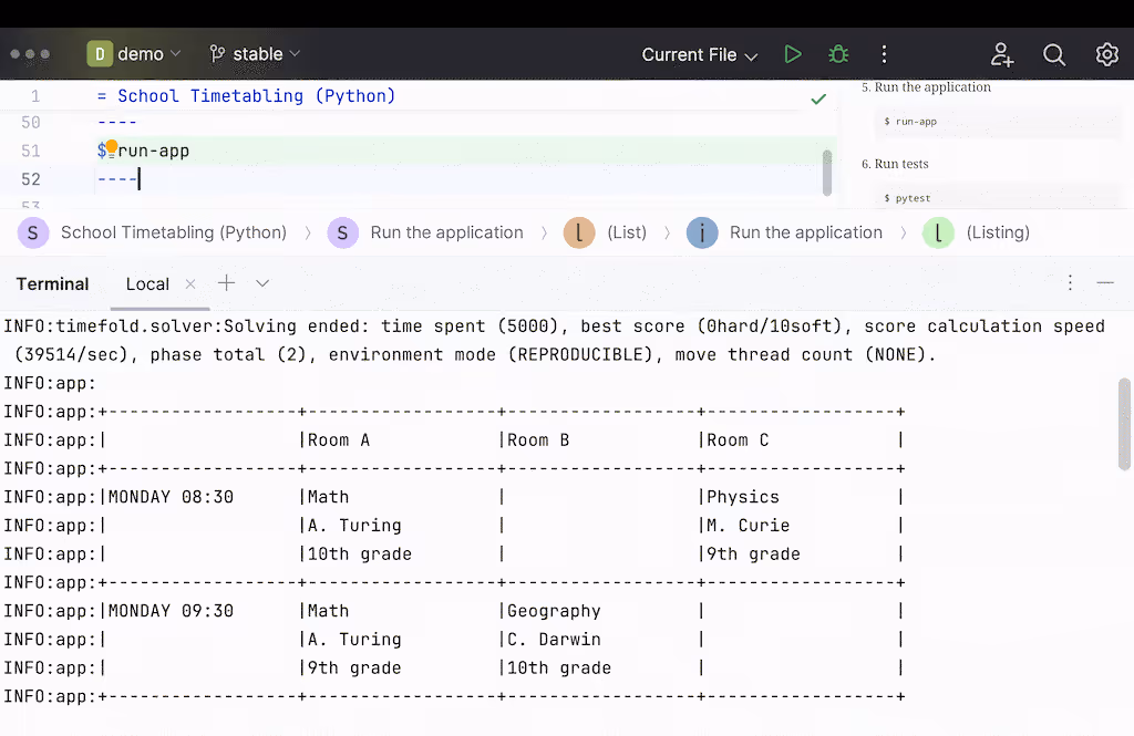
$ run-app

If you have questions, don’t hesitate to ask on StackOveflow. If you find an issue, report it in a GitHub issue.

Join the community

Join us in the community and start a GitHub discussion. To learn more about planning optimization, visit our website or follow us on Youtube.

At Timefold, our mission has always been to simplify the complexity of planning optimization and make it accessible to a wider audience. We started this journey with our Java solver, empowering developers to tackle NP-hard problems with ease. Today, we are thrilled to announce a major milestone: the release of our Python solver.

Why Python?

Python is a powerful, versatile, and widely-used programming language, particularly popular among data scientists, analysts, and developers. Its simplicity and readability make it an ideal choice for translating real-world constraints into code. By introducing a Python solver, we are expanding our reach and making planning optimization accessible to a larger community of developers who prefer Python over Java.

Benefits of the Timefold Python Solver

1. Ease of Use

Our Python solver simplifies the process of planning optimization by allowing developers to write their planning model directly in Python. This eliminates the need for writing complex mathematical equations, making it easier to translate real-world constraints into code.

2. Accessibility

With Python being a common language in data science and machine learning communities, the Python solver opens up our technology to a new audience. Data scientists and analysts can now leverage the power of Timefold without needing to switch to a different programming language.

3. Integration with Existing Tools

Python’s extensive ecosystem includes a variety of libraries and frameworks that can seamlessly be put into a workflow with our solver. Whether you are using pandas for data manipulation, NumPy for numerical computations, or any other Python library, our solver fits right into your workflow.

4. Flexibility

The Python solver is designed to be flexible and adaptable, allowing you to model complex planning problems with ease. Whether you are dealing with employee scheduling, field service routing, or maintenance scheduling, our solver can handle it all.

Important note: Alpha Release

Please not that our Python solver is currently in Alpha. The API set is not stable and it will likely change until we reach the Beta Phase. We are actively seeking feedback to help us refine and improve the Python Solver.

Getting Started with the Python Solver

We understand that getting started with a new tool can be daunting, so we have prepared comprehensive documentation and tutorials to guide you through the process. Our documentation covers everything from installation and setup to advanced usage and integration with other tools.

Visit this URL to access our Python solver and start optimizing your planning problems today. Our team is dedicated to supporting you every step of the way, so don’t hesitate to reach out with any questions or feedback.

Join the Conversation

We believe in the power of community and are excited to engage with you. Share your experiences, ask questions, and connect with other users in our community forums. Follow us on social media for the latest updates, tips, and success stories.

Conclusion

The release of our Python solver marks a significant step forward in our mission to make planning optimization accessible to all. We are excited to see how our community will leverage this new tool to solve complex planning problems and drive innovation in their fields.

Install Timefold Python Solver on PyPi: https://pypi.org/project/timefold-solver/

About Timefold

Timefold is dedicated to providing cutting-edge solutions for planning optimization. Our solvers are designed to simplify complex NP-hard problems, making them accessible to developers across various industries. With a focus on innovation and community, we strive to be the go-to platform for planning optimization and education.

By sharing this blog post, you can help us spread the word and make planning optimization accessible to a wider audience.

As more applications are moving towards cloud deployments, minimizing startup time is becoming more and more important. Read on to find out how to use Timefold Solver with Spring native images to reduce startup time in your application.

If you want to follow along, clone the Timefold quickstarts and change to the technology/java-spring-boot directory, which is already set up to support Spring native images:

git clone https://github.com/TimefoldAI/timefold-quickstarts.git
cd timefold-quickstarts/technology/java-spring-boot

Setup

You can modify your existing Spring applications to support building Spring native images by modifying your configuration.

MavenGradle

Add org.graalvm.buildtools:native-maven-plugin to your build plugins:

<build>
 <plugin>
     <groupId>org.graalvm.buildtools</groupId>
     <artifactId>native-maven-plugin</artifactId>
 </plugin>
</build>

Note: If you are not using spring-boot-starter-parent, you would need to configure executions for the process-aot goal from Spring Boot’s plugin and the add-reachability-metadata goal from the Native Build Tools plugin.

Building

Spring provides two ways of building a native image:

• Using Docker
• Using a locally installed GraalVM

Build using Docker

MavenGradle

mvn -Pnative spring-boot:build-image

This will produce an image tagged as docker.io/library/${name}:${version} where ${name} is the artifactId in Maven or the archivesBaseName in Gradle.

You can then run the image using Docker:

docker run --rm -p 8080:8080 docker.io/library/docker.io/library/timefold-solver-spring-boot-school-timetabling-quickstart:1.0-SNAPSHOT

Build using locally installed GraalVM

MavenGradle

mvn -Pnative native:compile

This will create an executable in target using the project’s artifactId as the name. The native image can then be run directly:

./target/timefold-solver-spring-boot-school-timetabling-quickstart

Benefits

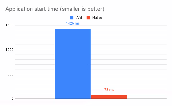
The primary benefit of native images is the massively reduced startup time:

./target/timefold-solver-spring-boot-school-timetabling-quickstart
...
20:40:44.888  INFO [main           ] Started TimetableSpringBootApp in 0.07 seconds (process running for 0.073)

Compared to running with a JVM:

java -jar target/timefold-solver-spring-boot-school-timetabling-quickstart-1.0-SNAPSHOT.jar
...
20:42:40.323  INFO [main           ] Started TimetableSpringBootApp in 1.216 seconds (process running for 1.426)

The native image started 20 times faster! This means a freshly started Kubernetes pod can respond to its first requests 20 times faster when a native image is used, changing an abysmal ~1 seconds wait time to a much more acceptable ~0.1 seconds wait time.

However, it is not all roses, since a native image is unable to perform various profiling based optimizations that a JVM can perform, reducing the speed of compute bound problems (such as solving):

./target/timefold-solver-spring-boot-school-timetabling-quickstart
...
20:58:43.064  INFO [pool-5-thread-1] Solving ended: ... score calculation speed (124774/sec) ...

Compared to running with a JVM:

java -jar target/timefold-solver-spring-boot-school-timetabling-quickstart-1.0-SNAPSHOT.jar
...
20:56:17.441  INFO [pool-2-thread-1] Solving ended: ... score calculation speed (213780/sec) ...

In a native image, Timefold Solver ran about 42% slower compared to a JVM run. This means to get to the same solution as a JVM run, the native image would need to run almost twice as long!

Important: Make sure to use GraalVM JDK 22 or above to generate the native image, which fixes a major performance regression involving record hashCode and equals.

Conclusion

It is easy to modify your existing Spring applications to make use of native images, allowing you to massively reduce startup time and thus respond to requests quicker on newly spawned Kubernetes pods. However, using native images currently prevents profiling based JIT optimizations, significantly impacting performance for compute bound tasks such as solving. If you have long-running solving tasks, consider running the solver in a separate application, which will allow you to gain the startup time benefits without affecting the performance of the solver.

Timefold offers continued support and further innovation.

As the original team behind OptaPlanner, we witnessed firsthand the challenges and limitations of continuing our mission to eliminate wasteful scheduling within Red Hat. The end of the Red Hat build of OptaPlanner and its evolution into an Apache project marks the end of an era. This moment signifies not just an end, but also a new beginning with Timefold.

What are the advised steps to safeguard your OptaPlanner project?

1. Reach Out Directly: Your first step is as simple as saying hello. Contact us via email at [email protected] or through our website's contact form. We guarantee a response within 24 hours on business days.
2. Discover what's new: We invite you to explore the enhancements and new features we’ve integrated into Timefold Solver by visiting our release notes page at https://timefold.ai/releases. Our solver is now twice as fast as OptaPlanner, thanks to the introduction of new features and critical bug fixes over the past year.
3. Upgrade to Timefold: Transitioning from OptaPlanner to Timefold is straightforward. We’ve designed the process to be completed in less than two minutes. Detailed instructions are available on our upgrade page, guiding you through every step.

All the knowledge and passion for planning optimization are now embodied in Timefold. Let us help you with continued support.

Bye Bye dummy vehicles, hello speed upgrade!

TL;DR: OptaPlanner and pre-1.8.0 Timefold users should upgrade for yet another significant performance boost.

Building on last year’s massive speed gains, we’re shifting to a higher gear.

Timefold 1.8.0 introduces support for planning list variables with unassigned values (nullable), enhancing scalability and efficiency.

Why should you care? It represents a big performance gain, especially when your operations doesn’t have enough resources to assign all necessary tasks to.

Your planning model benefits from this upgrade if it…

• Encounters Overconstrained Planning: struggling to assign all necessary tasks due to a shortage of resources.
• Implements the @PlanningListVariable annotation for managing planning list variables.
• Uses Multi-Resource Planning: Ideal for scenarios requiring multiple resources, like several vehicles or technicians at one location.

Impact of this upgrade

• OptaPlanner and pre-1.8.0: Models used "virtual vehicles" for tasks, which didn't scale well in multi-resource scenarios.
• Now, with 1.8.0: Introducing nullable planning list variables significantly improves scalability, showing remarkable performance in datasets with multi-resource visits.

Ok, what does the data say?

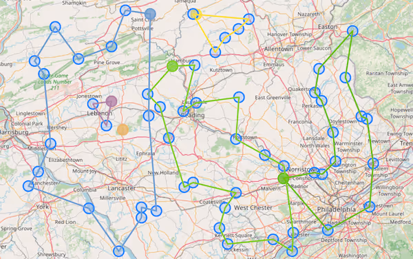
In the graph below we look at the impact on a Field Service Routing model with varying data set sizes. We look at the score calculation speed and benchmark versus the baseline, before Timefold 1.8.0 and after Timefold 1.8.0.

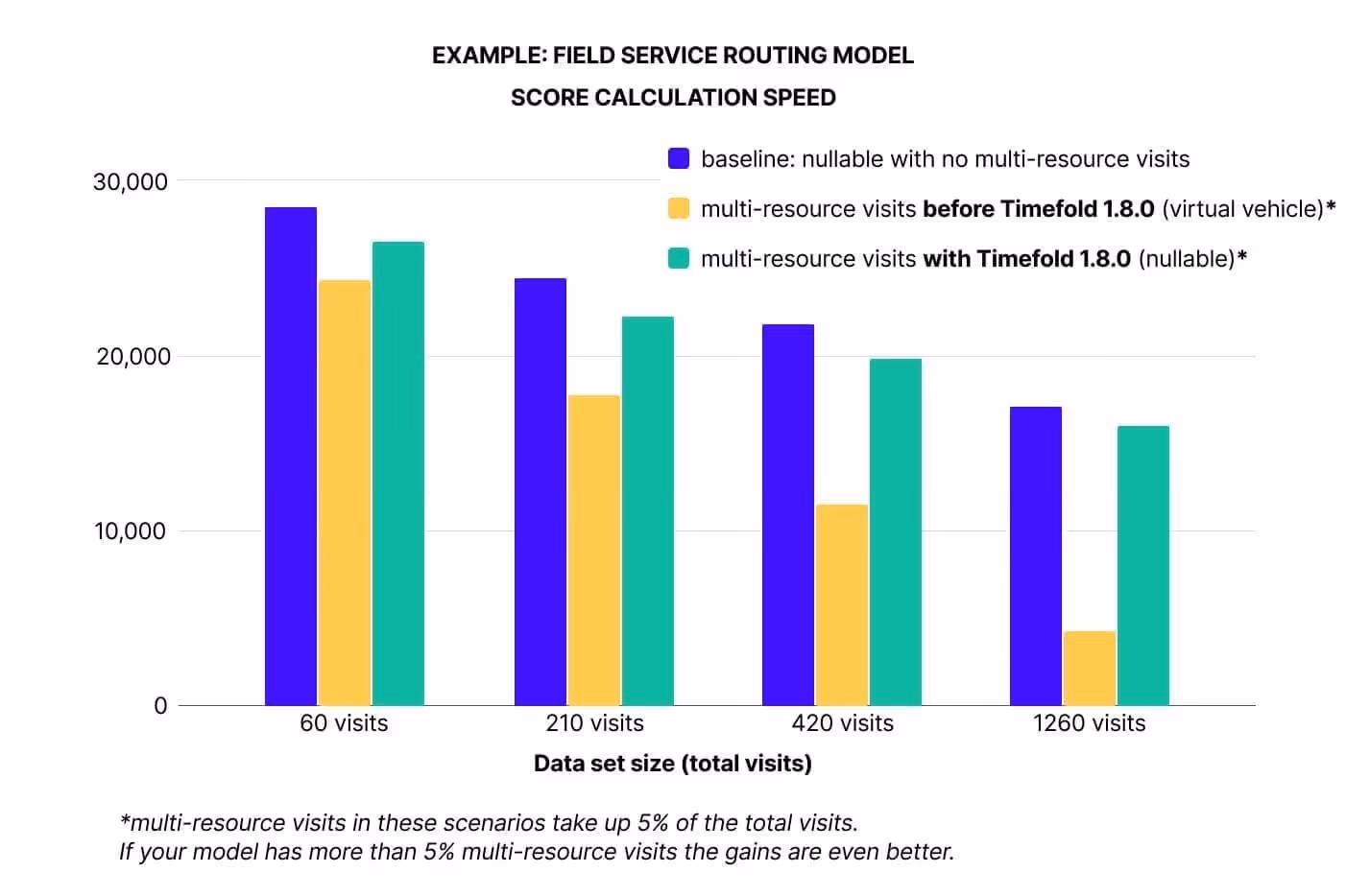
What is important for scalability is not the absolute value of the bar, but the speed with which it decreases with larger datasets.

The comparison of performance across different dataset sizes (from 60 to over 1200 visits) shows that nullable planning list variables maintain consistent performance, unlike virtual values that degrade with larger datasets.

This update is crucial for anyone dealing with overconstrained planning and multi-resource tasks, promising substantial scalability and efficiency improvements. Upgrade today

———

Case Study

Ecoprogram Flotte, an Italian leader in automotive logistics, needed a solution to optimize its transport planning. With Timefold, the company managed to build the best operational change ever for the company: a platform that makes vehicle deliveries and pick-ups more efficient and environmentally friendly.

Challenge

Streamlining the logistics to prepare and deliver 245,000 new cars to customers, while also managing the pickup of their used vehicles. This requires custom route planning for each driver, factoring in availability, residence, and more.

About Ecoprogram Flotte

• €258 million revenue (2024)
• 245000 car deliveries (2024)
• 850 employees, 300 drivers

Collaborates with international groups such as Arval, Gruppo Bnp Paribas,  ALD Automotive, Leasys, Unipol Rental, LeasePlan.

What Ecoprogram Flotte says about Timefold

“The Timefold platform is better than anything we have ever seen in the history of the company. Moreover, it fits in perfectly with our company’s sustainable ambitions.”

“The number of staff in the planning team decreased from five to one. We still see a big potential to further improve our planning and service delivery. This software enables us to stand out in our industry.”

Gregoire Chové - Managing Director

Read the full customer story

———

Blog

How fast is Java22?

With the release of Java 22 just around the corner, you may be wondering how it compares to Java 21 and whether you should upgrade. Additionally we compare it vs GraalVM.
Read the blog post

Advanced pinning in VRP. Reacting to sudden change

This article is focused on a more advanced pinning application for the Vehicle Routing Problem.
Read the blog post

———

Release notes

Timefold Solver Community Edition 1.8.0. full release notes

Spring is in the air, and so is another release of Timefold solver. This release is a significant leap forward, not just for our Community Edition users but for our Enterprise Edition clients as well, with each edition packed with features designed to supercharge your operations.

For our Community Edition, we have prepared the following features:

• List variables now allow for unassigned values. Read the beginning of this mail for more information.
• Spring Boot users among you can now easily generate native images, as was already possible for Quarkus.
• ConstraintVerifier can now test for justifications and indictments, allowing you to write tests that will give you even more confidence in your constraints than was possible before.
• We have exposed new metrics that allow you to better monitor the currently running solver(s).
• And last but not least, we've brought the usual bugfixes and dependency upgrades.

Exclusive Features for Enterprise Edition 1.8.0: Beyond the enhancements of the Community Edition, our Enterprise Edition users can access additional powerful features designed to significantly boost efficiency and performance.

• Automatic node sharing. Use cases with a large number of complex constraints may run as much as 30 % faster without any changes to your code.
• Nearby Selection can now be enabled with a single switch in your configuration, as opposed to the cumbersome configuration of old. If you're still not using Nearby Selection for your large routing problems, you're missing out on cost savings coming from significantly improved solutions!

Going forward, we will be publishing an Upgrade Recipe to let you know of any things you may or may not run into when upgrading to the latest version of Timefold Solver. It's a good read!

Here you can find all previous releases of Timefold Solver.

———

Latest Videos