Performance tips and tricks

Overview

The Solver will normally spend most of its execution time running score calculation, which is called in its deepest loops. Faster score calculation will return the same solution in less time with the same algorithm, which normally means a better solution in equal time.

Score calculation speed

After solving a problem, the Solver will log the score calculation speed per second. This is a good measurement of Score calculation performance, despite that it is affected by non-score calculation execution time. It depends on the problem scale of the problem dataset. Normally, even for large scale problems, it is higher than 1000, except if you are using EasyScoreCalculator.

When improving your score calculation, focus on maximizing the score calculation speed, instead of maximizing the best score. A big improvement in score calculation can sometimes yield little or no best score improvement, for example when the algorithm is stuck in a local or global optima. If you are watching the calculation speed instead, score calculation improvements are far more visible.

Furthermore, watching the calculation speed allows you to remove or add score constraints, and still compare it with the original’s calculation speed. Comparing the best score with the original’s best score is pointless: it’s comparing apples and oranges.

Incremental score calculation (with deltas)

When a solution changes, incremental score calculation (AKA delta based score calculation) calculates the delta with the previous state to find the new Score, instead of recalculating the entire score on every solution evaluation.

For example, when a shift in employee rostering is reassigned from Ann to Beth, it will not bother to check any other employees, since neither of them changed:

incrementalScoreCalculationEmployeeRostering

This is a huge performance and scalability gain. Constraint Streams API gives you this huge scalability gain without forcing you to write a complicated incremental score calculation algorithm.

Note that the speedup is relative to the size of your planning problem (your n), making incremental score calculation far more scalable.

Avoid calling remote services during score calculation

Do not call remote services in your score calculation, except if you are bridging EasyScoreCalculator to a legacy system. The network latency will kill your score calculation performance. Cache the results of those remote services if possible.

If some parts of a constraint can be calculated once, when the Solver starts, and never change during solving, then turn them into cached problem facts.

Pointless constraints

If you know a certain constraint can never be broken, or it is always broken, do not write a score constraint for it. For example, in vehicle routing, if you know that a vehicle can never visit a certain location, do not include it in the value range and it will never become a valid option for the solver to try.

Do not go overboard with this. If some datasets do not use a specific constraint but others do, just return out of the constraint as soon as you can. There is no need to dynamically change your score calculation based on the dataset.

In Constraint Streams, if you set constraint weight to zero, the constraint will be disabled and have no performance impact at all.

Built-in hard constraint

Instead of implementing a hard constraint, it can sometimes be built in. For example, if Lecture A should never be assigned to Room X, but it uses ValueRangeProvider on Solution, so the Solver will often try to assign it to Room X too (only to find out that it breaks a hard constraint). Use a ValueRangeProvider on the planning entity or filtered selection to define that Course A should only be assigned a Room different than X.

This can give a good performance gain in some use cases, not just because the score calculation is faster, but mainly because most optimization algorithms will spend less time evaluating infeasible solutions. However, usually this is not a good idea because there is a real risk of trading short-term benefits for long-term harm:

Many optimization algorithms rely on the freedom to break hard constraints when changing planning entities, to get out of local optima.
Both implementation approaches have limitations (feature compatibility, disabling automatic performance optimizations), as explained in their documentation.

Large cross-products

In order for constraints to scale well, it is necessary to limit the amount of data that flows through them. In Constraint Streams, it starts with joins. Consider a school timetabling problem, where a teacher must not have two overlapping lessons. This is how the lesson could look in Java:

    @PlanningEntity
    class Lesson {

        ...

        Teacher getTeacher() { ... }

        boolean overlaps(Lesson anotherLesson) { ... }

        boolean isCancelled() { ... }

        ...

    }

The simplest possible Constraint Stream we could write to penalize all overlapping lessons would then look like:

    constraintFactory.forEach(Lesson.class)
        .join(Lesson.class)
        .filter((leftLesson, rightLesson) ->
            !leftLesson.isCancelled()
	        && !rightLesson.isCancelled()
            && leftLesson.getTeacher()
                .equals(rightLesson.getTeacher())
            && leftLesson.overlaps(rightLesson))
        .penalize(HardSoftScore.ONE_HARD)
        .asConstraint("Teacher lesson overlap")

The join creates a cross-product between lessons, producing a match (also called a tuple) for every possible combination of two lessons, even though we know that many of these matches will not be penalized. This shows the problem in numbers:

Table 1. Fast growth of cross-product
Number of lessons	Number of possible pairs
10	100
100	10 000
1 000	1 000 000

To process a thousand lessons, the constraint first creates a cross-product of one million pairs, only to throw away pretty much all of them before penalizing. Reducing the size of the cross-product by half will therefore double the score calculation speed.

Filters before joins

As the example shows, canceled lessons are eventually filtered out after the join. Let’s instead remove them from the cross-product entirely. For the first lesson in the join, also called “left,” we put the cancellation check before the join like so:

    constraintFactory.forEach(Lesson.class)
        .filter(lesson -> !lesson.isCancelled())
        .join(Lesson.class)
        .filter((leftLesson, rightLesson) ->
            !rightLesson.isCancelled()
            && leftLesson.getTeacher() == rightLesson.getTeacher()
            && leftLesson.overlaps(rightLesson))
        ...

The canceled lessons are no longer coming in from the left, which reduces the cross-product. However, some canceled lessons are still coming in from the right through the join. They can be eliminated using a filtered nested stream:

    constraintFactory.forEach(Lesson.class)
        .filter(lesson -> !lesson.isCancelled())
        .join(
            constraintFactory.forEach(Lesson.class)
                .filter(lesson -> !lesson.isCancelled()))
        .filter((leftLesson, rightLesson) ->
            leftLesson.getTeacher() == rightLesson.getTeacher()
            && leftLesson.overlaps(rightLesson))
        ...

We’ve created a new Constraint Stream from Lesson, filtering before it entered our join. We have now applied the same improvement on both the left and right sides of the join, making sure it only creates a cross-product of lessons which we care about.

Joiners over filters

Filters are just a simple check if a tuple matches a predicate. If it does, it is propagated downstream, otherwise it is no longer evaluated. Each tuple needs to go through this check, and that means every pair of lessons will be evaluated. When a Lesson changes, all pairs with that Lesson will be wastefully re-evaluated. Let’s move the Teacher equality check moved from the final filter to a Joiner:

    constraintFactory.forEach(Lesson.class)
        .filter(lesson -> !lesson.isCancelled())
        .join(
            constraintFactory.forEach(Lesson.class)
                .filter(lesson -> !lesson.isCancelled()),
	        Joiners.equal(Lesson::getTeacher))
        .filter(Lesson::overlaps)
        ...

The constraint still says the same thing: a Lesson pair will only be sent downstream if they share the same Teacher. Unlike the filter, this brings the performance benefit of indexing. Now when a Lesson changes, only the pairs with the matching Teacher will be re-evaluated. So even though the cross-product remains the same, we are doing much less work processing it.

The final filter(Lesson::overlaps) now only performs one operation on the final cross product, and the number of Lesson pairs that get this far is already reduced as much as possible.

Removing more and earlier

If at all possible, the Joiner that will remove more tuples than the others should be put first. The size of cross-products will be the same, but the processing will happen more quickly.

Consider a new situation, where lessons also have rooms in which they happen. Although there are possibly dozens of teachers, there are only three rooms. Therefore, the join should look like this:

    constraintFactory.forEach(Lesson.class)
        .join(Lesson.class,
            Joiners.equal(Lesson::getTeacher),
            Joiners.equal(Lesson::getRoom))
    ...

This way, we first create “buckets” for each of the many teachers, and these buckets will only contain a relatively small number of lessons per room. If done the other way around, there would be a small number of large buckets, leading to much more iteration every time a lesson changes.

For that reason, it is generally recommended putting Joiners based on enum fields or boolean fields last.

Other score calculation performance tricks

Verify that your score calculation happens in the correct Number type. If you are making the sum of int values, do not sum it in a double which takes longer.
For optimal performance, use the latest Java version. We often see significant performance improvements by switching to new Java versions.
Always remember that premature optimization is the root of all evil. Make sure your design is flexible enough to allow configuration-based tweaking.

Score trap

Make sure that none of your score constraints cause a score trap. A trapped score constraint uses the same weight for different constraint matches, when it could just as easily use a different weight. It effectively lumps its constraint matches together, which creates a flatlined score function for that constraint. This can cause a solution state in which several moves need to be done to resolve or lower the weight of that single constraint. Some examples of score traps:

You need two doctors at each table, but you are only moving one doctor at a time. So the solver has no incentive to move a doctor to a table with no doctors. Punish a table with no doctors more than a table with only one doctor in that score constraint in the score function.
Two exams need to be conducted at the same time, but you are only moving one exam at a time. So the solver has to move one of those exams to another timeslot without moving the other in the same move. Add a coarse-grained move that moves both exams at the same time.

For example, consider this score trap. If the blue process moves from an overloaded computer to an empty computer, the hard score should improve. The trapped score implementation fails to do that:

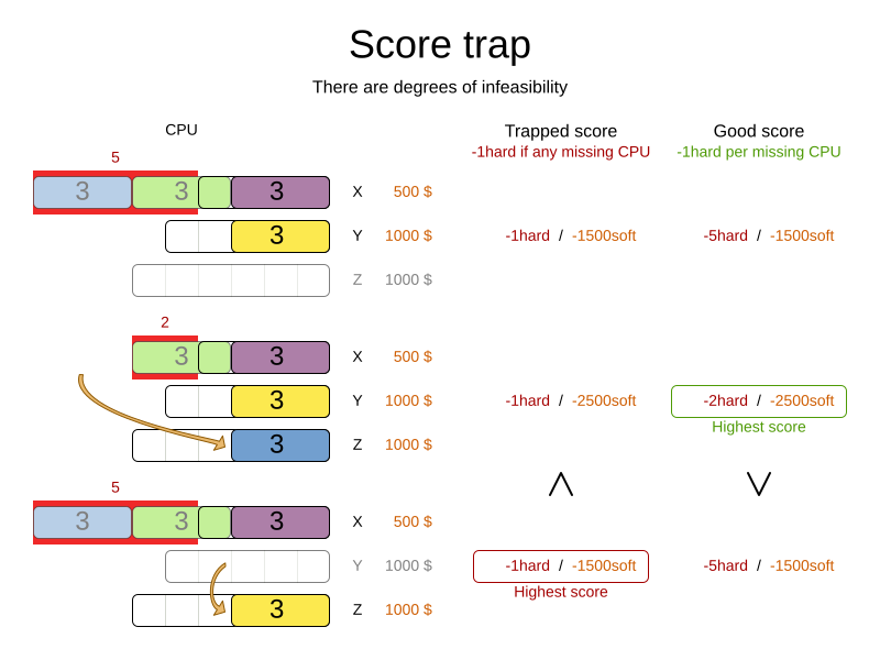
The Solver should eventually get out of this trap, but it will take a lot of effort (especially if there are even more processes on the overloaded computer). Before they do that, they might actually start moving more processes into that overloaded computer, as there is no penalty for doing so.

Avoiding score traps does not mean that your score function should be smart enough to avoid local optima. Leave it to the optimization algorithms to deal with the local optima. Avoiding score traps means to avoid, for each score constraint individually, a flatlined score function.

Always specify the degree of infeasibility. The business will often say "if the solution is infeasible, it does not matter how infeasible it is." While that is true for the business, it is not true for score calculation as it benefits from knowing how infeasible it is. In practice, soft constraints usually do this naturally and it is just a matter of doing it for the hard constraints too.

There are several ways to deal with a score trap:

Improve the score constraint to make a distinction in the score weight. For example, penalize -1hard for every missing CPU, instead of just -1hard if any CPU is missing.
If changing the score constraint is not allowed from the business perspective, add a lower score level with a score constraint that makes such a distinction. For example, penalize -1subsoft for every missing CPU, on top of -1hard if any CPU is missing. The business ignores the subsoft score level.
Add coarse-grained moves and union select them with the existing fine-grained moves. A coarse-grained move effectively does multiple moves to directly get out of a score trap with a single move. For example, move multiple items from the same container to another container.

`stepLimit` benchmark

Not all score constraints have the same performance cost. Sometimes one score constraint can kill the score calculation performance outright. Use the Benchmarker to do a one minute run and check what happens to the score calculation speed if you comment out all but one of the score constraints.

Fairness score constraints

Some use cases have a business requirement to provide a fair schedule (usually as a soft score constraint), for example:

Fairly distribute the workload amongst the employees, to avoid envy.
Evenly distribute the workload amongst assets, to improve reliability.

Implementing such a constraint can seem difficult (especially because there are different ways to formalize fairness), but usually the squared workload implementation behaves most desirable. For each employee/asset, count the workload w and subtract w² from the score.

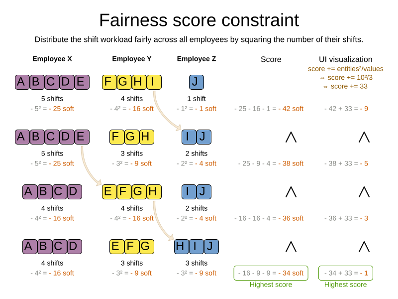
As shown above, the squared workload implementation guarantees that if you select two employees from a given solution and make their distribution between those two employees fairer, then the resulting new solution will have a better overall score. Do not just use the difference from the average workload, as that can lead to unfairness, as demonstrated below.

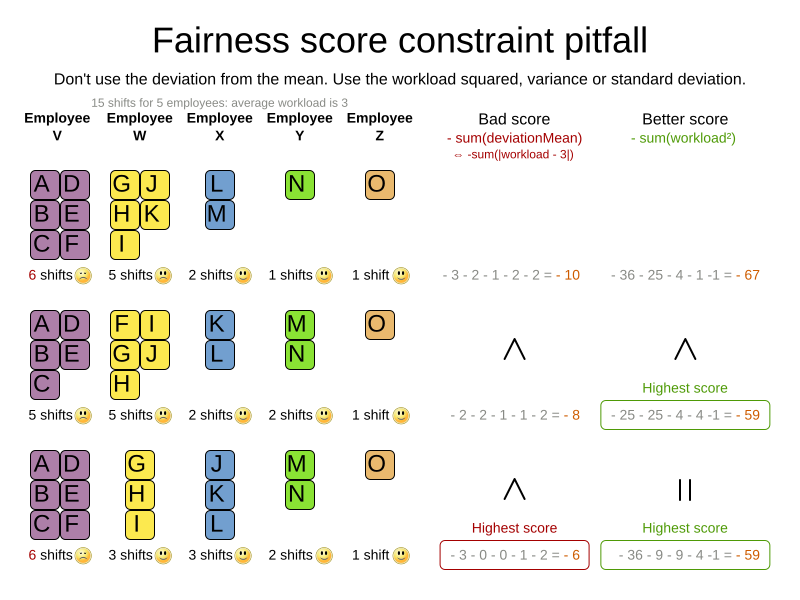
Instead of the squared workload, it is also possible to use the variance (squared difference to the average) or the standard deviation (square root of the variance). This has no effect on the score comparison, because the average will not change during planning. It is just more work to implement (because the average needs to be known) and trivially slower (because the calculation is a bit longer).

When the workload is perfectly balanced, the user often likes to see a 0 score, instead of the distracting -34soft in the image above (for the last solution which is almost perfectly balanced). To nullify this, either add the average multiplied by the number of entities to the score or instead show the variance or standard deviation in the UI.