Some of the users coming to Timefold from OptaPlanner might still be using score DRL to define their constraints. Since score DRL is the only thing we have not brought with us when we forked OptaPlanner, it is time to explain how to migrate from score DRL to Constraint Streams.

Constraint Streams (CS) is a modern full-featured API for writing Timefold Solver constraints, offering several benefits over score DRL:

• Developers do not need to learn any new language. CS is plain Java (or Kotlin).
• CS provides full IDE support including syntax highlighting and refactoring.
• CS provides comprehensive support for unit testing.
• In most use cases, CS performs considerably faster than score DRL.

Limits of this guide

CS and DRL are very similar in their approach to processing your data model. Because of this, migrating many parts of score DRL to CS is straight-forward, even mechanical. However, this guide does not help you if your score DRL uses the following constructs, because there is no direct mapping between DRL and CS in these cases:

• The DRL insertLogical() attribute allows information to be transferred between rules. This is not possible in CS, where each constraint is isolated and stands on its own. One typical use case for insertLogical() was detecting sequences of consecutive shifts in the Nurse Rostering example. This particular use case can be handled by using the consecutive constraint collector.
• The DRL right-hand side allows for arbitrary Java code execution that goes far beyond calculating the match weight. This is not possible in CS, where each constraint can only result in either a score reward or a penalty.

If you are using either of these constructs, we recommend that you first refactor them out of your DRL and then check back with this migration guide.

With that out of the way, let’s get the migration started.

Create and configure a ConstraintProvider class

In score DRL, all your constraints are typically written in a single text file, for example:

package org.optaplanner.examples.vehiclerouting.optional.score;
dialect "java"

import ...;

global HardSoftLongScoreHolder scoreHolder;

rule "vehicleCapacity"
   when
       ...
   then
       ...
end

...


In this file, each rule represents one or more constraints. In CS, the DRL file is replaced by standard Java source code:

package ai.timefold.solver.examples.vehiclerouting.score;

import ...;

public class VehicleRoutingConstraintProvider implements ConstraintProvider {

   @Override
   public Constraint[] defineConstraints(ConstraintFactory factory) {
       return new Constraint[] {
               vehicleCapacity(factory),
               ...
       };
   }

   protected Constraint vehicleCapacity(ConstraintFactory factory) {
       ...
   }

   ...
}


The method defineConstraints(…), a single method on the ConstraintProvider, lists all your constraints. Each constraint is then typically represented by a method.

Solver configuration

Quarkus and Spring users most likely do not need to worry about solver configuration. Just remove the score DRL and create a ConstraintProvider implementation.

In OptaPlanner’s solver configuration XML however, score DRL is configured by pointing the solver to the DRL file:

<solver>

 ...

 <scoreDirectorFactory>
   <scoreDrl>org/optaplanner/examples/vehiclerouting/optional/score/vehicleRoutingConstraints.drl</scoreDrl>
 </scoreDirectorFactory>

 ...

</solver>


Constraint Streams are selected by pointing the solver to an implementation of the ConstraintProvider interface from above:

<solver>

 ...

 <scoreDirectorFactory>
   <constraintProviderClass>ai.timefold.solver.examples.vehiclerouting.score.VehicleRoutingConstraintProvider</constraintProviderClass>
 </scoreDirectorFactory>

 ...

</solver>


Migrating trivial constraints

Many constraints follow a simple pattern of picking an entity and immediately penalizing it. Let’s look at an example from the field of vehicle routing:

rule "distanceToPreviousStandstill"
   when
       Customer(previousStandstill != null, $distanceFromPreviousStandstill : distanceFromPreviousStandstill)
   then
       scoreHolder.addSoftConstraintMatch(kcontext, - $distanceFromPreviousStandstill);
end


Here, each initialized Customer instance incurs a soft penalty equivalent to the value of its distanceFromPreviousStandstill field. Here’s how the same result is achieved in CS:

Constraint distanceToPreviousStandstill(ConstraintFactory factory) {
   return factory.forEach(Customer.class)
       .penalizeLong(HardSoftLongScore.ONE_SOFT, Customer::getDistanceFromPreviousStandstill)
       .asConstraint("distanceToPreviousStandstill");
}


Note that:

• forEach(Customer.class) serves the same purpose as Customer(…) in DRL.
• There is no need to check if a planning variable is initialized (previousStandstill != null), because forEach(…) does it automatically. If this behavior is not what you want, use forEachIncludingNullVars(…) instead.
• The right-hand side of the rule (the part after then) is replaced by a call to penalizeLong(…). The size of the penalty is now determined by the constraint weight (HardSoftLongScore.ONE_SOFT) and match weight (the call to a getter on Customer).

The match weight is a key difference between DRL and CS. In DRL, each rule adds a constraint match together with a total penalty. In CS, each constraint applies a reward or a penalty based on several factors:

• A penalty or reward. A penalty has a negative impact on the score, while a reward impacts the score positively.
• A constant constraint weight, such as HardSoftScore.ONE_SOFT, HardMediumSoftScore.ONE_HARD. Constraint weights can be either fixed or configurable.
• A dynamic match weight. This applies to any individual match and is typically specified by a lambda (for example customer -> customer.getDistanceFromPreviousStandstill()). If not specified, it defaults to 1.

The impact of each constraint match is calculated using the following formula:

(isReward ? 1 : -1) * (constraint weight) * (match weight)

Applying rewards instead of penalties

In the example above, score DRL applies a penalty by adding a negative constraint match, for example:

scoreHolder.addSoftConstraintMatch(kcontext, - $distanceFromPreviousStandstill).

CS makes this more explicit by using the keyword penalize instead of add…, while keeping the match weight positive:

penalizeLong(…, …, customer -> customer.getDistanceFromPreviousStandstill()).

You can accomplish a positive impact without changing the match weight if you replace penalize by reward :

rewardLong(…, …, customer -> customer.getDistanceFromPreviousStandstill()).

Applying different penalty types

In the example above, distanceFromPreviousStandstill is of the type long and therefore the DRL scoreHolder.addSoftConstraintMatch(kcontext, - $distanceFromPreviousStandstill) maps to the CS penalizeLong(…, …, customer -> customer.getDistanceFromPreviousStandstill()).

If the type was int, it would map to penalize(…) instead. Similarly, if the type was BigDecimal, it would map to penalizeBigDecimal(…). No types other than int, long, and BigDecimal are supported.

The same applies to rewards.

Applying configurable constraint weights

In some cases, such as in the Conference Scheduling example, constraint weights are specified in a @ConstraintConfiguration annotated class and not in the score DRL. The relevant right-hand side of the score DRL would look like this:

scoreHolder.penalize(kcontext, $penalty);

In CS, this situation maps to penalizeConfigurable(…) and similarly for rewards.

For more information, see penalties and rewards in Timefold Solver Documentation.

Migrating constraints with filters

In the vehicle routing field, we could also find the following rule:rule "distanceFromLastCustomerToDepot"
   when
       $customer : Customer(previousStandstill != null, nextCustomer == null)
   then
       Vehicle vehicle = $customer.getVehicle();
       scoreHolder.addSoftConstraintMatch(kcontext, - $customer.getDistanceTo(vehicle));
end


There are many similarities to the previous rule, but this time we penalize Customer only when the nextCustomer field is null. To do the same in CS, we introduce a filter(…)call where we check the return value of a getter for null.

Constraint distanceFromLastCustomerToDepot(ConstraintFactory factory) {
   return factory.forEach(Customer.class)
       .filter(customer -> customer.getNextCustomer() == null)
       .penalizeLong(HardSoftLongScore.ONE_SOFT,
           customer -> {
               Vehicle vehicle = customer.getVehicle();
               return customer.getDistanceTo(vehicle);
           })
       .asConstraint("distanceFromLastCustomerToDepot");
}


For more information, see filtering section in Timefold Solver Documentation.

Migrating eval(…)

The eval(…) construct allows us to execute an arbitrary piece of code that returns boolean. As such, it is functionally equivalent to the CS filter(…) construct as described previously. However, we discourage the use of eval(…) because executing custom code, such as calling external services or processing collections iteratively, is likely to slow your constraints down.

Migrating constraints with joins

Some constraints penalize based on a combination of entities or facts, such as in the NQueens example:

rule "Horizontal conflict"
   when
       Queen($id : id, row != null, $i : rowIndex)
       Queen(id > $id, rowIndex == $i)
   then
       scoreHolder.addConstraintMatch(kcontext, -1);
end


Here, we select a pair of different queens (second Queen.id greater than first Queen.id) which share the same row (second Queen.rowIndex equal to first Queen.rowIndex). Each pair is then penalized by 1.

Here’s how to do the same thing in CS, using a join(…) call with some Joiners:

Constraint horizontalConflict(ConstraintFactory factory) {
   return factory.forEach(Queen.class)
       .join(Queen.class,
           Joiners.greaterThan(Queen::getId),
           Joiners.equal(Queen::getRowIndex))
       .penalize(SimpleScore.ONE)
       .asConstraint("Horizontal conflict");
}


The Joiners.greaterThan(Queen::getId) statement is a way of expressing the DRL queen.id > $id statement in Java. Similarly, Joiners.equal(Queen::getRowIndex)represents the DRL queen.rowIndex == $i statement.

However, in this case, we can go further and use some CS syntactic sugar:

Constraint horizontalConflict(ConstraintFactory factory) {
   return factory.forEachUniquePair(Queen.class,
           equal(Queen::getRowIndex))
       .penalize(SimpleScore.ONE)
       .asConstraint("Horizontal conflict");
}


Using forEachUniquePair(Queen.class), the greaterThan(…) joiner is inserted automatically, and we only need to match the row indexes.

For more information, see joining in Timefold Solver Documentation.

Applying filters while joining

In certain cases, you might need to apply a filter while joining, such as in the case of the Conference Scheduling example:

rule "Talk prerequisite talks"
   when
       $talk1 : Talk(timeslot != null)
       $talk2 : Talk(timeslot != null,
               !getTimeslot().startsAfter($talk1.getTimeslot()),
               getPrerequisiteTalkSet().contains($talk1))
   then
       scoreHolder.penalize(kcontext,
               $talk1.getDurationInMinutes() + $talk2.getDurationInMinutes());
end


Note that the second Talk is only selected if its prerequisiteTalkSet contains the first Talk. Because there is no CS joiner for this specific operation yet, we need to use a generic filtering joiner:

Constraint talkPrerequisiteTalks(ConstraintFactory factory) {
   return factory.forEach(Talk.class)
       .join(Talk.class,
           Joiners.greaterThan(
                   talk1 -> talk1.getTimeslot().getEndDateTime(),
                   talk2 -> talk2.getTimeslot().getStartDateTime()),
           Joiners.filtering((talk1, talk2) -> talk2.getPrerequisiteTalkSet().contains(talk1)))
       .penalizeConfigurable(Talk::combinedDurationInMinutes)
       .asConstraint(TALK_PREREQUISITE_TALKS);
   }


Migrating large joins

CS only supports up to three joins natively. If you need four or more joins, refer to mapping tuples in Timefold Solver Documentation.

Migrating exists and not

The DRL exists keyword can be converted to CS much like the join above. Consider this rule from the Cloud Balancing example:

rule "computerCost"
   when
       $computer : CloudComputer($cost : cost)
       exists CloudProcess(computer == $computer)
   then
       scoreHolder.addSoftConstraintMatch(kcontext, - $cost);
end


Here, only penalize a computer if a process exists that runs on that particular computer. An equivalent constraint stream looks like this:

Constraint computerCost(ConstraintFactory constraintFactory) {
   return constraintFactory.forEach(CloudComputer.class)
       .ifExists(CloudProcess.class,
           Joiners.equal(Function.identity(), CloudProcess::getComputer))
       .penalize(HardSoftScore.ONE_SOFT, CloudComputer::getCost)
       .asConstraint("computerCost");
}


Notice how the ifExists(…) call uses the Joiners class to define the relationship between CloudProcess and CloudComputer.

For the use of the DRL not keyword, consider this rule from the Traveling Sales Person (TSP) example:

rule "distanceFromLastVisitToDomicile"
   when
       $visit : Visit(previousStandstill != null)
       not Visit(previousStandstill == $visit)
       $domicile : Domicile()
   then
       scoreHolder.addConstraintMatch(kcontext, - $visit.getDistanceTo($domicile));
end


A visit is only penalized if it is the final visit of the journey. The same can be achieved in CS using the ifNotExists(…) building block:

Constraint distanceFromLastVisitToDomicile(ConstraintFactory constraintFactory) {
   return constraintFactory.forEach(Visit.class)
       .ifNotExists(Visit.class,
           Joiners.equal(visit -> visit, Visit::getPreviousStandstill))
       .join(Domicile.class)
       .penalizeLong(SimpleLongScore.ONE, Visit::getDistanceTo)
       .asConstraint("Distance from last visit to domicile");
}


For more information on ifExists() and ifNotExists(), see conditional propagationin Timefold Solver Documentation.

Migrating accumulate

CS does not have a concept that maps mechanically to the DRL accumulate keyword. However, it does have a very powerful groupBy(…) concept. To understand the differences between the two, consider the following rule taken from the Cloud Balancing example:

rule "requiredCpuPowerTotal"
   when
       $computer : CloudComputer($cpuPower : cpuPower)
       accumulate(
           CloudProcess(
               computer == $computer,
               $requiredCpuPower : requiredCpuPower);
           $requiredCpuPowerTotal : sum($requiredCpuPower);
           $requiredCpuPowerTotal > $cpuPower
       )
   then
       scoreHolder.addHardConstraintMatch(kcontext, $cpuPower - $requiredCpuPowerTotal);
end


For each CloudComputer, it computes a sum of CPU power required by CloudProcessinstances ($requiredCpuPowerTotal : sum($requiredCpuPower)) running on that computer (CloudProcess(computer == $computer)), and only penalizes those computers where the total power required exceeds the power available ($requiredCpuPowerTotal > $cpuPower).

For comparison, let us now see how the same is accomplished in CS using groupBy(…):

Constraint requiredCpuPowerTotal(ConstraintFactory constraintFactory) {
   return constraintFactory.forEach(CloudProcess.class)
       .groupBy(
               CloudProcess::getComputer,
               ConstraintCollectors.sum(CloudProcess::getRequiredCpuPower))
       .filter((computer, requiredCpuPower) -> requiredCpuPower > computer.getCpuPower())
       .penalize(HardSoftScore.ONE_HARD,
           (computer, requiredCpuPower) -> requiredCpuPower - computer.getCpuPower())
       .asConstraint("requiredCpuPowerTotal");
   }


First, we select all CloudProcess instances (forEach(CloudProcess.class)). Then we apply groupBy in two steps:

1. We split the processes into buckets ("groups") by their computer (CloudProcess::getComputer). If two or more processes have the same computer, they belong to the same group.
2. For each such group, we apply a ConstraintCollectors.sum(…) to get a sum total of power required by all processes in such group.

The result of that operation is a pair ("tuple") of facts: a CloudComputer and an intrepresenting the sum total of power required by all processes running on that computer. We then take all such tuples and filter(…) out all those where the sum total is <= that computer’s available power. Finally, we penalize the positive difference between the required power and the available power, the overconsumption.

As you can see, groupBy(…) accomplishes the same result, but goes about it differently. This is why mapping DRL accumulate to CS groupBy, while always possible, is not necessarily straight-forward or mechanical.

For more information on groupBy(…), see grouping and collectors in Timefold Solver Documentation.

Conclusion

Users of Timefold Solver can no longer rely on score DRL to define their constraints. After migration to Constraint Streams, your constraints are likely to perform faster and be easier to maintain. Migrating most types of constraints to Constraint Streams is straightforward.

We have just released Timefold Solver 0.8.42. With this release, Timefold Solver 0.8 has reached End Of Life. Read on to find out why we are doing this, and what it means for you.

What is End Of Life?

End Of Life (EOL) means that Timefold will no longer provide support for Timefold Solver 0.8. There will be no new releases from the 0.8 branch, no more bugfixes and no more security updates. Upgrade to Timefold Solver 1.x to continue to receive updates.

Why has Timefold Solver 0.8 reached End Of Life?

Timefold Solver 0.8 is built on technologies which have themselves reached their respective EOL. Spring Boot 2’s final release is 2.7.18, and the final release of Quarkus 2 is 2.16.12.Final. Without support from these projects, Timefold can no longer provide users of Timefold Solver 0.8 with security updates.

What does this mean for you?

At the time of writing, Timefold Solver 1.4.0 is the current stable release of Timefold Solver. It contains the latest innovations, as well as all available bugfixes and the most recent security updates. It will be supported for many years to come. If you’re already on Timefold Solver 1.x, you’re all set.

Upgrading to Timefold Solver 1.x

The process to upgrade to latest Timefold Solver consists of several steps. First, upgrade your codebase to the latest Timefold like so:

Note that:

• Timefold Solver 1.x, as well as Spring Boot 3 and Quarkus 3, requires Java 17 or higher.
• Timefold Solver 1.x does not support scoreDRL, nor is it upgraded automatically. If you’re still using the legacy scoreDRL from OptaPlanner 7.x, which was already deprecated in OptaPlanner 8, please upgrade to Constraint Streams first.

Next steps depend on whether your project uses Spring Boot or Quarkus:

• If your project uses Spring Boot, follow the Spring Boot 3 migration guide to upgrade from Spring Boot 2 to Spring Boot 3.
• If your project uses Quarkus, follow the Quarkus 3.0 migration guide to upgrade from Quarkus 2 to Quarkus 3.
• If your project uses neither of these, skip these steps.

Having completed these steps, you are now on the latest Timefold Solver and you can enjoy all the latest features and bugfixes. Should you encounter any issues during the upgrade process, kindly contact us on Github and we will investigate.

Timefold customers can also contact our support directly.

Conclusion

Timefold Solver 0.8 has reached End of Life (EOL). Please upgrade to Timefold Solver 1.x now, to receive the latest and greatest features and bugfixes.

Zurich - Ghent - Swiss-based e-switch Solutions and Timefold announce a partnership to optimize maintenance and service management.

About e-switch Solutions

Founded in 1999: e-switch Solutions is a leading solutions provider, specializing in maintenance and service management. Offering Mobile SAP solutions which are adopted by leading companies like Deutsche Bahn, Siemens, Airport Zürich or Scottish Power.

e-switch Solutions‘ The Visual Planning Board® for dispatchers is an ideal solution for efficient scheduling featuring seamless integration with SAP and Real-Time updates. Their mobile solution, mCompanion®, supports technicians on-site throughout the entire process chain and is available on all leading mobile platforms. Additionally, their checklist tool, mcCheckList®, aids with digital checklists to help adhere to and document work processes, integrated with SAP data.

e-switch Solutions fuels maintenance scheduling with Timefold

The Visual Planning Board® by e-switch Solutions features an innovative OTS module (Optimized Task Scheduling), originally based on the OptaPlanner open-source project.

Recognizing the advancements and superior capabilities of Timefold, the evolution of OptaPlanner, e-switch Solutions strategically opted to integrate Timefold into their platform. Ensuring that e-Switch remains at the forefront of service and maintenance management innovation.

The strategic partnership with Timefold is an important step for the future. Our SAP expertise in the area of service and maintenance, supplemented by the solver component from Timefold, expands our Visual Planning Board with a powerful optimizer for automatic resource planning. In view of the growing demand for optimizer solutions, we are confident that e-switch is optimally equipped for the future.

Thorsten Waldner from e-switch Solutions

About Timefold

Timefold created an AI-powered, Open Source planning technology platform designed to enhance operational efficiency across various industries. Timefold offers tools to solve complex planning problems through mathematical optimization and makes it accessible for developers.

Diverse Industry Applications: Off the shelf, Timefold’s customizable planning models cater for common, yet complex planning problems. Ranging from Maintenance Scheduling, Vehicle Routing, to Employee Scheduling and Production line scheduling. These models can be tailored to fit the specific needs and nuances of individual use cases.

Proprietary with Maven Repository: This option includes a proprietary but open-source accessible platform, available through the Timefold Maven repository with solver jars and a quickstarts repo.

Managed Solution with Container Registry: Alternatively, Timefold provides a managed solution available via its container registry, including Docker images and helm charts, complemented by an API service.

Gurobi and Timefold Solver are mathematical optimization solvers. Both are fast and scalable solvers, used across the globe by a large user base in production. They have similarities, but also differences.

This comparison is written by the Timefold team to guide you through the fundamental differences in these technologies. We aim to present correct and truthful information. However, it’s important to acknowledge our natural bias towards Timefold Solver.

License and community

Both Gurobi and Timefold Solver are created by companies with dedicated team of optimization experts. Both have a large community, high-quality documentation and a rich set of examples.

Gurobi

Gurobi is paid, proprietary software.

To get started, contact Gurobi for a free evaluation license, then read the docs or start from the examples.

Timefold Solver

Timefold Solver Community is open source software under the Apache License, which allows free usage in commercial software.

To get started, read the docs or clone the quickstarts repo on GitHub.

Timefold Solver Enterprise is paid, proprietary software, that adds support and high-scalability features. This comparison covers only the features in the free, open source edition.

Define a model

Both Gurobi and Timefold Solver require you to define your model with optimization variables, so the mathematical optimization software knows which decisions it needs to make.

Gurobi

Gurobi supports several types of optimization variables, such as booleans, integers and floating point numbers. You can define your planning model in those types.

For example, you can use addVar(BINARY) to model the assignment of a particular employee to a particular shift:

// Input
Model model = ...
Variable[][] assignments = new Variable[shifts.size()][employees.size()];
for (int s = 0; s < shifts.size(); s++) {
   for (int e = 0; e < employees.size(); e++) {
       assignments[s][e] = model.addVar(BINARY);
   }
}
... // Add constraints to enforce no shift is assigned to multiple employees

// Solve
model.solve();

// Output
for (int s = 0; s < shifts.size(); s++) {
   for (int e = 0; e < employees.size(); e++) {
       if (assignments[s][e].get() > 0.99) {
           print(shifts[s] + " is assigned to " + employees[e]);
       }
   }
}

Timefold Solver

Timefold Solver supports any type of optimization variables, including your custom classes (Employee, Vehicle, …​) and standard classes (Integer, BigDecimal, LocalDate, …​). You typically define your planning model in your own domain classes.

For example, you can use @PlanningVariable on your Shift.employee field to model the assignment of an employee to a shift:

@PlanningEntity
class Shift { // User defined class
   ... // id, date, start time, required skills, ...

   @PlanningVariable
   Employee employee;
}
@PlanningSolution
class TimeTable { // User defined class
   List<Employee> employees;
   List<Shift> shifts;
}

// Input
Timetable timetable = new Timetable(shifts, employees);

// Solve
timetable = Solver.solve(timetable);

// Output
for (Shift shift : timetable.shifts) {
   print(shift + " is assigned to " + shift.employee);
}

None of these classes (Shift, Employee and Timetable) exist in Timefold itself: you define and shape them. Your code naturally represents employees as instances of the Employee class, shifts as instances of the Shift class, and so forth.

Timefold Solver supports Object-Oriented Programming (OOP) input, including polymorphism.

Search space comparison

In the code above for employee scheduling, Gurobi uses boolean variables and Timefold uses employee variables.

This has an effect on the search space:

• Gurobi creates a boolean variable for every (shift, employee) combination. Given 2000 shifts and 100 employees, that’s an array of 200 000 elements.
• On the other hand, Timefold Solver creates an Employee variable for every Shift. Given 2000 shifts and 100 employees, that’s an array of 2000 elements.

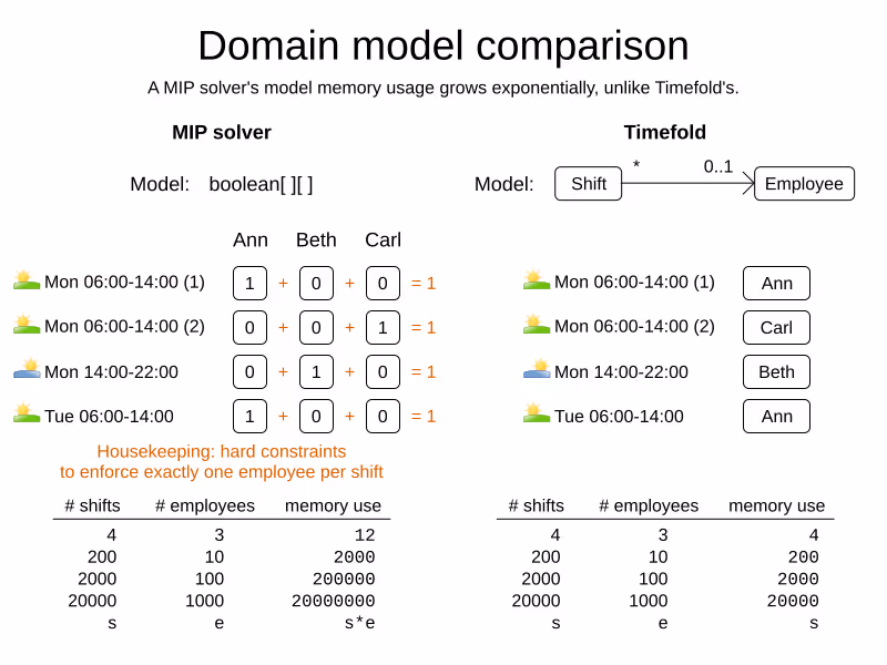
The Timefold model naturally enforces the one shift per employee hard constraint by design, the Gurobi model implements it.

Constraints

Both Gurobi and Timefold Solver have a rich API to define your constraints.

Gurobi

Gurobi constraints are implemented as mathematical equations.

For example, to assign at most one shift per day, you add an equation s1 + s2 + s3 <= 1 for all shifts on day 1, an equation s4 + s5 <= 1 for all shifts on day 2, and so forth:

for (int e = 0; e < employees.size(); e++) {
   for (int d = 0; d < dates.size(); d++) {
       Expression expr = ...
       for (int s = 0; s < shifts.size(); s++) {
           // If the shift is on the date
           if (shifts[s].date == dates[d])) {
               expr.addTerm(1.0, assignments[s][e]);
           }
       }
       model.addConstraint(expr, LESS_EQUAL, 1.0);
   }
}

Timefold Solver

Timefold Solver constraints are implemented as programming code.

For example, to assign at most one shift per day, select every pair of Shift instances that have the same date and the same employee, to penalize matching pairs as a hard constraint:

// For every shift ...
constraintFactory.forEach(Shift.class)
   // ... combined with any other shift ...
   .join(Shift.class,
       // ... on the same date ...
       equal(shift -> shift.date),
       // ... assigned to the same employee ...
       equal(shift -> shift.employee))
   // ... penalize one broken hard constraint per pair.
   .penalize(HardSoftScore.ONE_HARD)
   .asConstraint("One shift per day");

Timefold’s ConstraintStreams API uses a Functional Programming (FP) approach, so it can run delta calculations under the hood for maximum scalability and performance.

Constraints can reuse existing code. For example, because date is an instance of LocalDate (a Date and Time API), you can use LocalDate.isDayOfWeek() to select 2 shifts on the same day of week:

       // ... on the same day of week ...
       equal(shift -> shift.date.getDayOfWeek())

Date and times arithmetic is notoriously difficult, because of Daylight Saving Time (DST), timezones, leap years and other intricacies. Timefold allows you to directly use any 3th-party API (such as LocalDate) in your constraints.

Besides the equal() joiner, Timefold provides lessThan(), greaterThan(), lessThanOrEqual(), greaterThanOrEqual(), overlapping(), etc. It automatically applies indexing (hashtable techniques) on joiners for performance.

It has higher level abstractions. For example, select two overlapping shifts with the overlapping() joiner (even if they start or end at different times):

       // ... that overlap ...
       overlapping(shift -> shift.startDateTime, shift -> shift.endDateTime)

Besides the join() construct, Timefold supports filter(), groupBy(), ifExists(), ifNotExists(), map(), etc.

For example, allow employees that can work double shifts to work double shifts by filtering out all employees that work double shifts with a filter():

// For every shift ...
constraintFactory.forEach(Shift.class)
   // ... assigned to an employee that does not work double shifts ...
   .filter(shift -> !shift.employee.worksDoubleShifts)
   // ... combined with any other shift ...
   .join(Shift.class,
       equal(shift -> shift.date),
       // ... assigned to that same employee that does not work double shifts ...
       equal(shift -> shift.employee))
   .penalize(HardSoftScore.ONE_HARD)
   .asConstraint("One shift per day");

The groupBy() construct supports count(), sum(), average(), min(), max(), toList(), toSet(), toMap(), etc. You can also plug in custom collectors.

For example, don’t assign more than 10 shifts to any employee by counting their shifts with count():

constraintFactory.forEach(Shift.class)
   // Group shifts by employee and count the number of shifts per employee ...
   .groupBy(shift -> shift.employee, count())
   // ... if more than 10 shifts for one employee ...
   .filter((employee, shiftCount) -> shiftCount > 10)
   // ... penalize as a hard constraint ...
   .penalize(HardSoftScore.ONE_HARD,
           // ... multiplied by the number of excessive shifts.
           (employee, shiftCount) -> shiftCount - 10)
   .asConstraint("Too many shifts");

Timefold Solver has no linear limitations.

For example, avoid overtime and distribute it fairly by penalizing the number of excessive hours squared:

constraintFactory.forEach(Shift.class)
   // Group shifts by employee and sum the shift duration per employee ...
   .groupBy(shift -> shift.employee, sum(shift -> shift.getDurationInHours()))
   // ... if an employee is working more hours than his/her contract ...
   .filter((employee, hoursTotal) -> hoursTotal > employee.contract.maxHours)
   // ... penalize as a soft constraint of weight 1000 ...
   .penalize(HardSoftScore.ofSoft(1000),
           // ... multiplied by the number of excessive hours squared.
           (employee, hoursTotal) -> {
                   int excessiveHours = hoursTotal - employee.contract.maxHours;
                   return excessiveHours * excessiveHours;
           })
   .asConstraint("Too many shifts");

This penalizes outliers more. It automatically load balances overtime in fair manner across the employees, whenever possible.

Timefold Solver also supports positive constraints: use reward() instead of penalize(). You can mix positive and negative constraints.

Timefold Solver supports weighting constraints dynamically per dataset.

Scoring

Gurobi

Gurobi supports 2 score levels: hard constraints as constraints and soft constraints as an objective function that returns a floating point number.

Gurobi uses floating point arithmetic internally to solve. It minimizes rounding errors by ordering its arithmetic operations intelligently. By default, Gurobi tolerates going over hard constraints by margin of a 0.000001 to ignore compounded rounding errors.

Timefold Solver

Timefold Solver supports extra score levels beyond hard and soft constraints. For example, HardMediumSoftScore allows to prioritize medium operational constraints (such as assign all shifts) over soft financial constraints (such as reduce cost). Without resorting to multiplication with a big number.

Timefold Solver supports to weight constraints dynamically per dataset without rebuilding the entire model. For example to make the soft constraint fairness in dataset A twice as important as in dataset B.

Timefold Solver includes a Score Analysis API to break down a score per constraint.

Timefold Solver does not suffer from numerical instability because it doesn’t rely on floating point arithmetic internally for constraint validation.

Cloud and Integration

Gurobi

Gurobi Cloud offers a paid service to run models on Azure and AWS clouds.

Timefold Solver

Timefold Solver has integration modules for Spring, Quarkus and JSON (de)serialization. It supports native compilation for serverless use cases that need to start up in milliseconds.

Timefold (company) offers a paid Field Service Routing API and Employee Scheduling API, as well as a paid version of Timefold Solver with Enterprise Features such as Nearby Selection and Multi-Threading.

Page updated on 12th of November 2025 to beter differentiate between Timefold (the company) and Timefold Solver.

Google OR-Tools and Timefold Solver are open source mathematical optimization solvers. Both are fast and scalable solvers, used across the globe by a large user base in production. They have similarities, but also differences.

This comparison is written by the Timefold team to guide you through the fundamental differences in these technologies. We aim to present correct and truthful information. However, it’s important to acknowledge our natural bias towards Timefold.

Number of solvers

OR-Tools

OR-Tools has individual solvers for Constraint Programming (CP), Mixed-Integer Programming (MIP), Vehicle Routing (VRP) and Graph Algorithms. Each solver has its own API, tailored to a specific set of use cases.

OR-Tools comes with a set of examples for each of these solvers to learn the different APIs easily.

Timefold Solver

Timefold Solver is one solver, with a unified API that handles any use case with any combination of constraints. It can solve hybrid problems, such as Vehicle Routing with a constraint to distribute the workload fairly across drivers (a typical constraint of Employee Rostering).

Timefold Solver comes with a GitHub quickstarts repo that provides a starting point for each use case, such as Vehicle Routing with Time Windows.

Define a model

Define a model (non vehicle routing)

Both OR-Tools CP and Timefold Solver require you to define your model with optimization variables, so the mathematical optimization software knows which decisions it needs to make.

OR-Tools CP

OR-Tools’s CP solver supports 3 types of optimization variables: booleans, integers and floating point numbers. You can define your planning model in those types.

For example, you can use model.newBoolVar() to model the assignment of a particular employee to a particular shift:

// Input
CpModel model = ...
IntVar[][] assignments = new IntVar[shifts.size()][employees.size()];
for (int s = 0; s < shifts.size(); s++) {
   for (int e = 0; e < employees.size(); e++) {
       assignments[s][e] = model.newBoolVar(...);
   }
}
... // Add constraints to enforce no shift is assigned to multiple employees

// Solve
solver.solve(model);

// Output
for (int s = 0; s < shifts.size(); s++) {
   for (int e = 0; e < employees.size(); e++) {
       if (value(assignments[s][e]) == 1L) {
           print(shifts[s] + " is assigned to " + employees[e]);
       }
   }
}

Timefold Solver

Timefold Solver supports any type of optimization variables, including your custom classes (Employee, Vehicle, …​) and standard classes (Integer, BigDecimal, LocalDate, …​). You typically define your planning model in your own domain classes.

For example, you can use @PlanningVariable on your Shift.employee field to model the assignment of an employee to a shift:

@PlanningEntity
class Shift { // User defined class
   ... // Shift id, date, start time, required skills, ...

   @PlanningVariable
   Employee employee;
}

class Employee { // User defined class
 ... // Name, skills, ...
}

@PlanningSolution
class TimeTable { // User defined class
   List<Employee> employees;
   List<Shift> shifts;
}

// Input
Timetable timetable = new Timetable(shifts, employees);

// Solve
timetable = Solver.solve(timetable);

// Output
for (Shift shift : timetable.shifts) {
   print(shift + " is assigned to " + shift.employee);
}

None of these classes (Shift, Employee and Timetable) exist in Timefold Solver itself: you define and shape them. Your code naturally represents employees as instances of the Employee class, shifts as instances of the Shift class, and so forth.

Timefold Solver supports Object-Oriented Programming (OOP) input, including polymorphism.

Search space comparison

In the code above for employee scheduling, OR-Tools uses boolean variables and Timefold Solver uses employee variables.

This has an effect on the search space:

• OR-Tools’s CP solver creates a boolean variable for every (shift, employee) combination. Given 2000 shifts and 100 employees, that’s an array of 200 000 elements.
• On the other hand, Timefold Solver creates an Employee variable for every Shift. Given 2000 shifts and 100 employees, that’s an array of 2000 elements.

The Timefold Solver model naturally enforces the one shift per employee hard constraint by design, the OR-Tools CP model implements it.

Define a vehicle routing model

OR-Tools Vehicle Routing

OR-Tools has a separate API for Vehicle Routing based on OR-Tools’s RoutingModel class which comes with a fixed number of constraints out-of-the-box:

// Input
RoutingIndexManager manager = new RoutingIndexManager(locationListSize, vehicleListSize, 0);
RoutingModel routingModel = new RoutingModel(manager); // OR-Tools defined class
routingModel.setArcCostEvaluatorOfAllVehicles(...);
routingModel.addDimensionWithVehicleCapacity(...);

// Solve
Assignment assignment = routingModel.solve();

// Output
for (int i = 0; i < vehiclesCount; i++) {
   long index = routingModel.start(i);
   print("Vehicle " + i + ": ");
   while (!routing.isEnd(index)) {
     print(manager.indexToNode(index) + ", ");
     index = solution.value(routing.nextVar(index));
   }
}

Timefold Solver

Timefold Solver solves Vehicle Routing like any other planning problem, but provides building blocks for Vehicle Routing, such as list variables (and shadow variables to calculate the arrival time):

@PlanningEntity
class Vehicle { // User defined class
   ... // start time, start location, capacity, skills, ...

   @PlanningListVariable
   List<Visit> visits;
}

class Visit { // User defined class
   ... // location, demand, time window(s), ...
}

// Input
VehicleRoutePlan plan = new VehicleRoutePlan(vehicles, visits);

// Solve
plan = Solver.solve(plan);

// Output
for (Vehicle vehicle : plan.vehicles) {
   print(vehicle + ": " + vehicle.visits);
}

On the base model, you can add complex constraints, such as floating lunch breaks, multi-vehicle visits and any other custom constraint.

Constraints

OR-Tools CP

OR-Tools’s CP solver constraints are implemented as mathematical equations.

For example, to assign at most one shift per day, you add an equation s1 + s2 + s3 <= 1 for all shifts on day 1, an equation s4 + s5 <= 1 for all shifts on day 2, and so forth:

for (int e = 0; e < employees.size(); e++) {
   for (int d = 0; d < dates.size(); d++) {
       IntVar[] vars = new IntVar[...];
       int i = 0;
       for (int s = 0; s < shifts.size(); s++) {
           // If the shift is on the date
           if (shifts[s].date == dates[d])) {
               vars[i++] = assignments[s][e];
           }
       }
       model.addLessOrEqual(LinearExpr.sum(vars), 1);
   }
}

OR-Tools Vehicle Routing

OR-Tool’s VRP solver comes with a fixed number of constraints out-of-the-box, such as time windows. You can find all the available constraints on the RoutingModel class.

Timefold Solver

Timefold Solver constraints are implemented as programming code.

For example, to assign at most one shift per day, select every pair of Shift instances that have the same date and the same employee, to penalize matching pairs as a hard constraint:

// For every shift ...
constraintFactory.forEach(Shift.class)
   // ... combined with any other shift ...
   .join(Shift.class,
       // ... on the same date ...
       equal(shift -> shift.date),
       // ... assigned to the same employee ...
       equal(shift -> shift.employee))
   // ... penalize one broken hard constraint per pair.
   .penalize(HardSoftScore.ONE_HARD)
   .asConstraint("One shift per day");

Timefold’s ConstraintStreams API uses a Functional Programming (FP) approach, so it can run delta calculations under the hood for maximum scalability and performance.

Constraints can reuse existing code. For example, because date is an instance of LocalDate (a Date and Time API), you can use LocalDate.isDayOfWeek() to select 2 shifts on the same day of week:

       // ... on the same day of week ...
       equal(shift -> shift.date.getDayOfWeek())

Date and times arithmetic is notoriously difficult, because of Daylight Saving Time (DST), timezones, leap years and other intricacies. Timefold Solver allows you to directly use any 3th-party API (such as LocalDate) in your constraints.

Besides the equal() joiner, Timefold provides lessThan(), greaterThan(), lessThanOrEqual(), greaterThanOrEqual(), overlapping(), etc. It automatically applies indexing (hashtable techniques) on joiners for performance.

It has higher level abstractions. For example, select two overlapping shifts with the overlapping() joiner (even if they start or end at different times):

       // ... that overlap ...
       overlapping(shift -> shift.startDateTime, shift -> shift.endDateTime)

Besides the join() construct, Timefold Solver supports filter(), groupBy(), ifExists(), ifNotExists(), map(), etc.

For example, allow employees that can work double shifts to work double shifts by filtering out all employees that work double shifts with a filter():

// For every shift ...
constraintFactory.forEach(Shift.class)
   // ... assigned to an employee that does not work double shifts ...
   .filter(shift -> !shift.employee.worksDoubleShifts)
   // ... combined with any other shift ...
   .join(Shift.class,
       equal(shift -> shift.date),
       // ... assigned to that same employee that does not work double shifts ...
       equal(shift -> shift.employee))
   .penalize(HardSoftScore.ONE_HARD)
   .asConstraint("One shift per day");

The groupBy() construct supports count(), sum(), average(), min(), max(), toList(), toSet(), toMap(), etc. You can also plug in custom collectors.

For example, don’t assign more than 10 shifts to any employee by counting their shifts with count():

constraintFactory.forEach(Shift.class)
   // Group shifts by employee and count the number of shifts per employee ...
   .groupBy(shift -> shift.employee, count())
   // ... if more than 10 shifts for one employee ...
   .filter((employee, shiftCount) -> shiftCount > 10)
   // ... penalize as a hard constraint ...
   .penalize(HardSoftScore.ONE_HARD,
           // ... multiplied by the number of excessive shifts.
           (employee, shiftCount) -> shiftCount - 10)
   .asConstraint("Too many shifts");

Timefold Solver has no linear limitations.

For example, avoid overtime and distribute it fairly by penalizing the number of excessive hours squared:

constraintFactory.forEach(Shift.class)
   // Group shifts by employee and sum the shift duration per employee ...
   .groupBy(shift -> shift.employee, sum(shift -> shift.getDurationInHours()))
   // ... if an employee is working more hours than his/her contract ...
   .filter((employee, hoursTotal) -> hoursTotal > employee.contract.maxHours)
   // ... penalize as a soft constraint of weight 1000 ...
   .penalize(HardSoftScore.ofSoft(1000),
           // ... multiplied by the number of excessive hours squared.
           (employee, hoursTotal) -> {
                   int excessiveHours = hoursTotal - employee.contract.maxHours;
                   return excessiveHours * excessiveHours;
           })
   .asConstraint("Too many shifts");

This penalizes outliers more. It automatically load balances overtime in fair manner across the employees, whenever possible.

Timefold Solver also supports positive constraints: use reward() instead of penalize(). You can mix positive and negative constraints.

Scoring

OR-Tools CP

OR-Tools’s CP solver supports 2 score levels: hard constraints as constraints and soft constraints as an objective function that returns a floating point number.

OR-Tools Vehicle Routing

OR-Tools’s Vehicle Routing solver only supports the hard and soft constraints in the RoutingModel class.

Timefold Solver

Timefold Solver supports extra score levels beyond hard and soft constraints. For example, HardMediumSoftScore allows to prioritize medium operational constraints (such as assign all shifts) over soft financial constraints (such as reduce cost). Without resorting to multiplication with a big number.

Timefold Solver supports to weight constraints dynamically per dataset without rebuilding the entire model. For example to make the soft constraint fairness in dataset A twice as important as in dataset B.

Timefold Solver includes a Score Analysis API to break down a score per constraint.

Timefold Solver does not suffer from numerical instability because it doesn’t rely on floating point arithmetic internally for constraint validation.

Cloud and Integration

Both OR-Tools and Timefold Solver run on Linux, Mac and Windows. Both can run locally and in the cloud.

OR-Tools

Google Research offers a paid Operations Research API in the cloud based on OR-Tools.

Timefold Solver

Timefold Solver has integration modules for Spring, Quarkus and JSON (de)serialization. It supports native compilation for serverless use cases that need to start up in milliseconds.

Timefold (company) offers a paid Field Service Routing API and Employee Scheduling API, as well as a paid version of Timefold Solver with Enterprise Features such as Nearby Selection and Multi-Threading.

License, support and community

Both OR-Tools and Timefold Solver Community are open source software under the Apache License, which allows free usage in commercial software. In both cases, the code is open on GitHub.

OR-Tools

OR-Tools is developed by a small team at Google with help from the open source community.

To get started, go the OR-Tools website and follow the get started guide.

Timefold Solver

Timefold Solver is developed by Timefold BV with help from the open source community. Timefold BV is a company that lives and breathes planning optimization.

To get started, read the docs or clone the quickstarts repo on GitHub.

This comparison covered only the features in the free, open source edition.

Page updated on 12th of November 2025 to beter differentiate between Timefold (the company) and Timefold Solver.

Have you ever received a solution from the Solver and wondered what -3hard/-11softactually means? Or had to explain it to your end-users? Now, you can just show it to them. In Timefold Solver 1.4.0, you can break down the score of a solution into constraints and constraint matches, to make it understandable for your end-users.

Let’s take a closer look and find out what’s new in another exciting monthly release of Timefold Solver.

Break down the score per constraint

We expand on our existing functionality by making score explanations easier to use than ever before. Here’s how you start using this new feature:

// First, we get some solution from the solver. Nothing new here, business as usual.
SolverJob<Timetable, ...> solverJob = solverManager.solve(...);
Timetable timetable = solverJob.getFinalBestSolution();

// Now that we have the timetable, we can analyze the score.
ScoreAnalysis<HardSoftScore> scoreAnalysis = solutionManager.analyze(timetable);

The ScoreAnalysis object holds the total score of the analyzed solution, and a breakdown of the score per constraints. This allows you to easily see which constraints are impacting your solution the most.

System.out.println("Total score: " + scoreAnalysis.score());
scoreAnalysis.constraintMap().forEach((constraint, constraintAnalysis) -> {
  System.out.println("              Constraint: " + constraint);
  System.out.println("Score for the constraint: " + constraintAnalysis.score());
});

You can break the score down even further, by going deeper into the ConstraintAnalysis object. Each such object contains a list of matches, which are the individual violations of the constraint. This allows you to see which planning entities or values are causing the constraint to be violated. also called a justification.

for (MatchAnalysis<HardSoftScore> match: constraintAnalysis.matches()) {
   System.out.println("        Match score: " + match.score());
   System.out.println("Match justification: " + match.justification());
}

With this data structure, you have the full overview of your planning solution and how it was scored by Timefold Solver. But we did not stop there!

Score analysis is JSON-friendly

In today’s world, what good are excellent backend APIs if you cannot send the results over the wire to the frontend? We’ve got you covered. The ScoreAnalysis object is JSON-friendly, which means you can easily serialize it and send it over the wire. In Quarkus and Spring Boot, the ScoreAnalysis object will automatically serialize to JSON such as this:

{
 "score" : "0hard/4soft",
 "constraints" : [ {
   "package" : "org.acme.schooltimetabling.domain",
   "name" : "Teacher time efficiency",
   "score" : "0hard/5soft",
   "matches" : [ {
     "score" : "0hard/1soft",
     "justification" : {
       "lessonId1": 5,
       "lessonId2": 17,
       "teacher": "I. Jones"
     },
     ... ] }
   }, {
   "package" : "org.acme.schooltimetabling.domain",
   "name" : "Student group subject variety",
   "score" : "0hard/-1soft",
   "matches" : [ ... ]
   } ]
}

We see the score is made up of two constraints here, each with their own score and matches. The frontend can then easily display the score breakdown to the user, such as this:

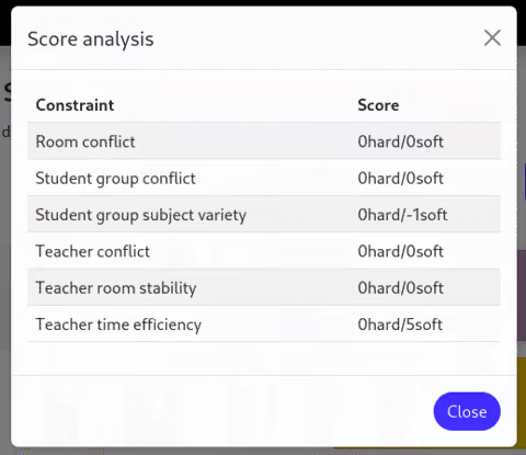
Note that in this case, we have chosen not to display the individual constraint matches to make the visualization simpler. In a more detail-oriented view, you may choose to display the individual matches as well.

See it in action

The code snippets above are taken from the School Timetabling quickstart in the Timefold Quickstarts Github repository. You can run the quickstart locally by following a few short steps. Clone it today and experience Timefold Solver for yourself!

Comparing solutions to one another

In addition to the new score explanation functionality, we have also made it easier to compare two solutions to one another. You can use the same score analysis functionality above to compare two solutions.

The ScoreAnalysis object has a diff(ScoreAnalysis otherScoreAnalysis) method which, when called, returns a new ScoreAnalysis object. This object holds the differences between the two solutions. It shows the difference in score and the difference in individual constraints, down to every single constraint match.

Check out our docs to learn everything there is about understanding the score.

What else is new?

Besides the features above, we have brought the usual battery of bug fixes and performance improvements. With Timefold Solver 1.4.0, you can enjoy slightly faster Constraint Streams and an even more stable experience. We also upgraded Quarkus, Spring and other dependencies to their latest versions.

We are also happy to have been included in Spring Initializr, making your getting started experience with Spring Boot and Timefold Solver even easier!

Conclusion

Timefold Solver continues full steam ahead. The new explainable score functionality is a great addition, and a feature much requested by our users. Upgrade now to get the best release yet!

In the world of Java and Kotlin development, Spring Boot is often the go-to choice for building a wide range of applications. Now, imagine if this reliable companion could also handle complex planning problems like Vehicle Routing, Shift Scheduling, Order Picking, Assembly Line scheduling, … Well, thanks to Timefold, it now can!

Spring Boot and start.spring.io: A Developer’s Paradise

For developers, starting a new project often involves a visit to start.spring.io. Creating Spring Boot projects with just a few clicks. It’s where innovation begins, and now, it’s where intelligent planning solutions come to life. With the integration of Timefold Solver, developers can effortlessly incorporate planning optimization into their Spring Boot projects.

Timefold Solver: Your planning solution

At its core, Timefold Solver is an embeddable code library tailor-made for planning problems. It’s not your typical off-the-shelf software; it’s a versatile engine that can be seamlessly integrated into your applications. Timefold Solver isn’t bound by a single use case; it adapts to your specific needs, making it the perfect companion for developers who demand flexibility and precision.

Solving the toughest Planning Problems

Planning challenges come in various forms and sizes, from optimizing vehicle routes to crafting complex schedules. Timefold tackles them all. It’s the trusted ally that developers turn to when they need to automate and streamline planning processes. With Timefold, you’re not just coding; you’re crafting intelligent solutions.

How to Get Started

1. Visit start.spring.io: Begin your journey by creating a Spring Boot project. It’s the same trusted starting point you know and love, but now with an extra layer of intelligence.
2. Add Timefold: In the project generation wizard, simply include Timefold as a dependency. This step will ensure that your Spring Boot application is equipped to handle intricate planning challenges.
3. Coding with Timefold: Once your project is set up, dive into the code and explore the capabilities of Timefold. Create PlanningEntities and PlanningSolutions, and let Timefold do the heavy lifting when it comes to solving planning puzzles.

Visit our Spring Boot Java Quick Start Guide and solve complex planning problems such as vehicle routing, shift scheduling, school timetabling, etc.

Benefits Galore

• Integrating Timefold into Spring Boot brings a host of benefits to developers:
• Efficiency: Say goodbye to manual planning; Timefold automates the process.
• Precision: Solve complex optimization challenges with ease.
• Flexibility: Adapt Timefold to your specific planning needs.
• Time Savings: Let Timefold handle the intricacies while you focus on core development.

Conclusion: A Bright Future for Spring Boot Developers

With the addition of Timefold to the Spring Boot ecosystem, developers now have a powerful ally in solving intricate planning problems. Whether it’s optimizing routes, scheduling shifts, or crafting timetables, Timefold and Spring Boot together offer an intelligent, developer-friendly solution.

With the release of Java 21 just around the corner, you may be wondering how it compares to Java 17 and whether you should upgrade. Here at Timefold, so were we. Read on to find out how Timefold Solver performs on Java 21, compared to Java 17.

But first, let’s get some things out of the way.

What is Java 21 and how to get it

Java 21 is a new release of the Java platform, the trusty programming language that Timefold Solver is written in. It brings a bunch of new features, as well as the usual bugfixes and smaller improvements.

Java 21 will be generally available on September 19, 2023, but you can already try it out using the release candidate builds. We find that the easiest way to get started with Java 21 is to use SDKMAN, and that is what did as well. (See the end of this post for the specific versions and hardware used.)

Like Java 17 before it, Java 21 is a long-term support (LTS) release; it will stick around for quite a while. It is therefore a good idea to start using it as soon as possible and see if it works for you.

For Timefold Solver, that means making sure the entire codebase continues to work flawlessly on Java 21, as well as running some benchmarks to ensure our users can expect at least the same performance as before. Let’s get started on that.

Micro-benchmarks

We’ll start with score director micro-benchmarks, which we use regularly to establish the impact of various changes on the performance of Constraint Streams. These benchmarks do not run the entire solver; rather, they focus exclusively on the score calculation part of the solver.

They are implemented using Java Microbenchmark Harness (JMH), and they run in many Java Virtual Machine (JVM) forks and with sufficient warmup. This gives us a good level of confidence in the results. In fact, the margin of error on these numbers is only ± 2%.

Here is the Constraint Streams performance on Java 21 vs. Java 17:

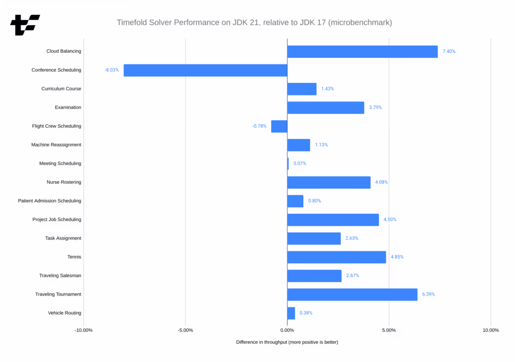
Most cases show a small performance improvement when switching to Java 21. The "Conference Scheduling" benchmark is the only outlier, and with some extra work on the solver we can likely get the performance of that benchmark to improve as well.

It should be noted that we ran these benchmarks with ParallelGC as the garbage collector (GC), instead of the default G1GC. Later in this post we’ll explain why.

Real-world benchmarks

Now that we’ve seen the micro-benchmarks, it’s time to compare them to real-world solver performance. This includes the entire solver, not just the score calculation part.

We ran the solver manually in 10 different JVM forks, and used the median score calculation speed. We selected a subset of the available benchmarks, to keep the run time short; the selection is representative of the entire benchmark suite in terms of heuristics used and code paths exercised. Once again, ParallelGC is used as the garbage collector. Here are the results:

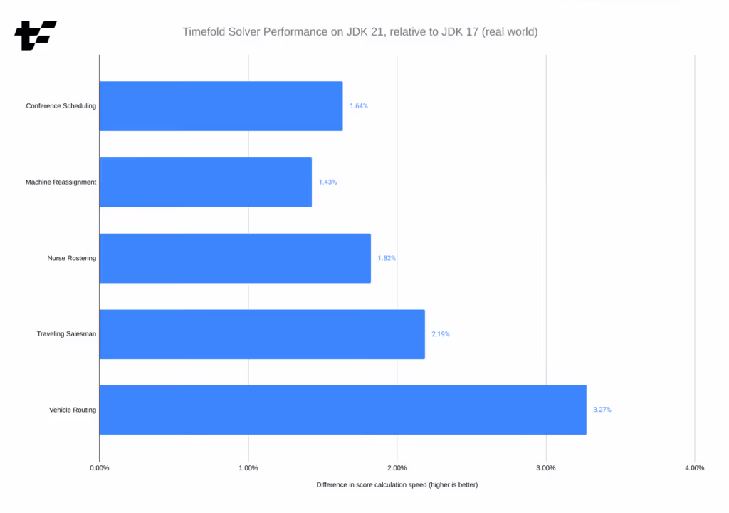
There are no surprises here. We see small performance improvements across the board, confirming the results of the micro-benchmarks. Compared to the micro-benchmarks, "Conference Scheduling" no longer registers as an outlier, which is interesting and will serve as another data point in our investigation into that possible regression.

Since we haven’t established a formal interval of confidence for these large benchmarks, we can’t say with certainty that the improvements are statistically significant. However, the fluctuations observed between runs have been small enough to give us confidence in the results.

Why ParallelGC?

In the years that we’ve been working with the Timefold Solver and its predecessor, OptaPlanner, we’ve found that ParallelGC is the best garbage collector for the solver. This should not be surprising - ParallelGC is tailored for high throughput, and the solver is 100 % CPU-bound. G1GC (the default garbage collector) is instead tailored for low latency, and that makes a considerable difference. However, things change and we occasionally need to challenge our assumptions. Is ParallelGC still the best GC for the solver?

The following chart shows the difference in performance between G1GC (the baseline) and ParallelGC. And since Java 21 introduced generational ZGC, another GC aiming for low latency, we thought it would be interesting to include that as well.

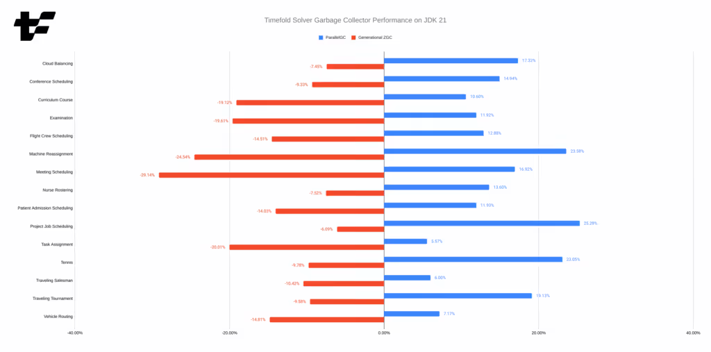
The results (obtained by the micro-benchmarks from earlier) are clear:

• ParallelGC continues to be the best GC for the solver.
• G1GC comes second, but it’s considerably slower.
• ZGC is by far the worst of the three.

The situation may change if we increased the heap size available to the JVM as ParallelGC does not scale well with large heaps, but with -Xmx1G, it is the clear winner. (And 1GB of heap is more than enough for many use cases of Timefold Solver.)

Conclusion

In this post, we’ve shown that:

• Timefold Solver 1.1.0 works perfectly fine with Java 21, no changes are needed.
• Switching to Java 21 may bring a small performance improvement to your Timefold Solver application, but your mileage may vary slightly.
• ParallelGC continues to be the best garbage collector for the solver.

We encourage you to try Java 21 and make the switch. It is free after all, and you’ll be able to enjoy the latest and greatest Java platform.

Appendix A: Reproducing the results

These benchmarks use Timefold Solver 1.1.0, the latest version at the time of writing.

All benchmarks were run on Fedora Linux 38, with Intel Core i7-12700H CPU and 32 GB of RAM. We used OpenJDK Runtime Environment Temurin-17.0.8+7 (build 17.0.8+7) (available as 17.0.8-tem on SDKMAN) and OpenJDK Runtime Environment (build 21+35-2513) (available as 21.ea.35-open on SDKMAN).

Source code of the micro-benchmarks can be found in my own personal repository. The real-world benchmarks were run using timefold-solver-benchmark, this configuration and a simple script. (You’ll need timefold-solver-examples on the classpath.) All data used for the charts can be found in this spreadsheet.

The vehicle routing problem (VRP) is a popular academic optimization problem with numerous variants.

While you can map the vehicle routing problem to real-world tasks like planning deliveries or optimizing itineraries for field service technicians, very often you have to deal with at least one additional constraint: customers' availabilities.

This post will show you how to solve the vehicle routing problem using Timefold Solver.

VRP with time windows

Let’s start by defining the problem. Same as the vanilla VRP, the task is to plan routes of N vehicles to visit M customers to minimize the driving time. The additional complexity comes from customers' availability in limited time windows. If the vehicle arrives at the destination too early, it has to wait, which is suboptimal. If it arrives too late, it’s even worse as the planned visit has to be rescheduled to some other day and all the mileage driven comes in vain.

Domain model

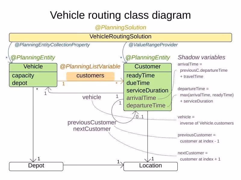
The domain model takes advantage of the @PlanningListVariable: the Vehicle is the @PlanningEntity with a list of Customer instances to visit. The @PlanningListVariable enables the use of a few build-in shadow variables:

• @InverseRelationShadowVariable that points from the Customer to the assigned Vehicle.
• @PreviousElementShadowVariable and @NextElementShadowVariable that point to the previous and the next customer in the list respectively.

To calculate the arrival time at each customer, the model relies on the arrivalTimeshadow variable that is updated by the ArrivalTimeUpdatingVariableListener every time the previousCustomer or the vehicle changes.

Constraints

The constraints are implemented using the Constraint Streams API and you can see them in the VehicleRoutingConstraintProvider.java.

Service must be finished in time

Providing the service to the customer also takes time, expressed by the serviceDuration. Of course, the service duration counts towards the customer’s availability. This is a hard constraint.

protected Constraint serviceFinishedAfterDueTime(ConstraintFactory factory) {
   return factory.forEach(Customer.class)
           .filter(Customer::isServiceFinishedAfterDueTime)
           .penalizeLong(HardSoftLongScore.ONE_HARD,
                   Customer::getServiceFinishedDelayInMinutes)
           .asConstraint("serviceFinishedAfterDueTime");
}

Minimize travel time

This is a soft constraint that penalizes the time spent driving per every vehicle, knowing the distances between individual locations.

protected Constraint minimizeTravelTime(ConstraintFactory factory) {
   return factory.forEach(Vehicle.class)
           .penalizeLong(HardSoftLongScore.ONE_SOFT,
                   Vehicle::getTotalDrivingTimeSeconds)
           .asConstraint("minimizeTravelTime");
}

Wait a second, where do we make sure we don’t arrive too early? The serviceFinishedAfterDueTime constraint does it for us, just indirectly. The more time vehicles spend waiting, the fewer customers they can visit without arriving too late.

Try for yourself

1. git clone [email protected]:timefoldai/timefold-quickstarts.git
2. cd timefold-quickstarts/use-cases/vehicle-routing
3. mvn quarkus:dev
4. Open a browser and navigate to http://localhost:8080
5. Click on the solve button

If you want to try your own dataset, use the REST API. Click the Guide in the top-level menu to learn how to get started.

Conclusion

The vehicle routing with time windows is a more practical variation of VRP, which we might translate to domains like field service technician or last mile delivery. You can solve all these using Timefold Solver.