Do you want to understand what OptaPlanner is doing while it is solving? Which decisions it makes? When? And why? Do you want to open the box and take a look inside? If so, keep reading.

The Age of Enlightenment centered on the use of reason and the evidence of the senses. Similarly, OptaPlanner enlightenment starts with the use of reason and the evidence in the logs.

OK. That’s enough philosophy for this article…​ It’s time to open the box. Take a look at the log for the school timetabling AI quickstart:

12:18:04 INFO Solving started: time spent (196), best score (-38init/0hard/0soft), environment mode (REPRODUCIBLE), move thread count (NONE), random (JDK with seed 0).
12:18:04 INFO Construction Heuristic phase (0) ended: time spent (330), best score (0hard/-11soft), score calculation speed (4358/sec), step total (19).
12:18:34 INFO Local Search phase (1) ended: time spent (30000), best score (0hard/10soft), score calculation speed (12786/sec), step total (26654).
12:18:34 INFO Solving ended: time spent (30000), best score (0hard/10soft), score calculation speed (12663/sec), phase total (2), environment mode (REPRODUCIBLE), move thread count (NONE).

This is a lot of information, even on the INFO level. Let’s investigate each nugget of information in there, one by one:

When did the solver run?

The log shows when the solver started and when it ended:

12:18:04 INFO Solving started ... ... 12:18:34 INFO Solving ended ...

That’s useful in complex applications with other log lines intertwined.

What is the solver doing?

It also displays what the solver did while solving:

12:18:04 INFO Solving started ... 12:18:04 INFO Construction Heuristic phase (0) ended ... 12:18:34 INFO Local Search phase (1) ended ... 12:18:34 INFO Solving ended ...

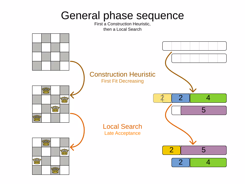
It ran two algorithm phases sequentially:

• Phase 0: a Construction Heuristic to provide an initial solution for the problem
• Phase 1: a Local Search to improve the solution further

Here’s an illustration of those phases on the N-Queens and the Cloud Balancing examples:

If the Local Search log line is missing (after the solver ends), the Construction Heuristic did not have enough time to initialize the entire solution, leaving no time for the Local Search algorithm. That returns an incomplete or infeasible solution.

Time spent

The log also exhibits how long each of those phases took, in milliseconds, relevant to the start of the solver:

12:18:04 INFO Solving started time spent (196) ...
12:18:04 INFO Construction Heuristic ended ... time spent (330) ...
12:18:34 INFO Local Search ended ... time spent (30000) ...
12:18:34 INFO Solving ended time spent (30000), ...

• The Solver initialization took 196 milliseconds.
• The Construction Heuristic took 330 - 196 = 134 milliseconds.
  • For big datasets, if the CH takes more than one minute, it’s worth investigating why, even if the solver runs for hours.
• The Local Search took 30000 - 330 = 29670 milliseconds.
  • LS gets the lion’s share of the time, as it should be.

Score quality

The log also reveals the solution quality after each algorithm:

INFO Solving started ... best score (-38init/0hard/0soft) ...
INFO Construction Heuristic ended ... best score (0hard/-11soft) ...
INFO Local Search ended ... best score (0hard/10soft) ...
INFO Solving ended ... best score (0hard/10soft) ...

• The starting score -38init/0hard/0soft indicates there are 38 unassigned planning variables. That’s because there are 19 lessons, each with 2 planning variables to initialize.
• The Construction Heuristic ends with a solution of score 0hard/-11soft, which is already feasible (no hard constraints broken). That’s not always the case.
• The Local Search improves the score further to score 0hard/10soft. That’s a difference of +21soft in 29 seconds.

Performance

There’s also performance information to discover in the log. First ensure it’s an apples-to-apples comparison:

12:18:04 INFO Solving started ... environment mode (REPRODUCIBLE), move thread count (NONE) ...
...
12:18:34 INFO Solving ended ... environment mode (REPRODUCIBLE), move thread count (NONE).

• If the environment mode is any ASSERT mode, performance is irrelevant, because the extra assertions are very expensive performance wise.
• The move thread count indicates how many extra CPU cores it can consume.
  • NONE means all move calculations happen inside the solver’s thread, so only 1 CPU is exploited.

Both of these affect the score calculation speed, which shows how many moves were evaluated, normalized per second, for the solver entirely, but also each phase separately:

12:18:04 INFO Solving started ...
12:18:04 INFO Construction Heuristic ended ... score calculation speed (4358/sec) ...
12:18:34 INFO Local Search ... score calculation speed (12786/sec) ...
12:18:34 INFO Solving ended ... score calculation speed (12663/sec) ...

• The Construction Heuristic evaluated over 4000 moves per second.
  • That’s actually pretty low, but it only ran for 134 milliseconds, so the overhead weighs in too much, lowering the number significantly. It should be run with a bigger dataset instead.
  • Normally, the score calculation speed of the Construction Heuristic is higher than that of the Local Search, because it’s faster to calculate the score when half of the entities aren’t initialized yet.
• The Local Search evaluated over 12000 moves per second.
  • That’s good. The LS score calculation speed should always be above 10 000 per second, even for big datasets.
  • Do note that it ran for 29 seconds and a JVM can take a minute to warm up.

Keep an eye on the score calculation when adding/editing constraints, running the solver for same amount of time (typically 1 minute), to discover performance bottlenecks early. For more accurate performance investigations, use optaplanner-benchmark which supports warming up.

Steps

In essence, both the Construction Heuristic phase and Local Search phase run a double loop:

  for (Step step : steps) { // Outer loop
      for (Move move : moves) { // Inner loop
          // Evaluate move
      }
      // Take step
  }

The outer, step loop executes the best move found by the inner, move loop. Of course, this is a gross simplification: there are dozens of orthogonal AI subsystems on top of it. It’s only the tip of the iceberg. But it’s an honest simplification.

The INFO log shows how many of these outer loop iterations both phases did:

...
12:18:04 INFO Construction Heuristic ended ... step total (19).
12:18:34 INFO Local Search ended ... step total (26654).
...

• The Construction Heuristic did 19 steps. That’s because there are 19 lessons in the dataset. Each step assigns one lesson.
• The Local Search did over 26 000 steps. It continues iterating until the termination condition is hit. Each step modifies (often improves) the current solution.

Turn on DEBUG logging to get a log line per step too:

INFO  Solving started: time spent (619), best score (-38init/0hard/0soft), environment mode (REPRODUCIBLE), move thread count (NONE), random (JDK with seed 0).
DEBUG     CH step (0), time spent (650), score (-36init/0hard/0soft), selected move count (30), picked move ([Biology(18) {null -> Room A}, Biology(18) {null -> MONDAY 09:30}]).
DEBUG     CH step (1), time spent (661), score (-34init/0hard/0soft), selected move count (30), picked move ([Chemistry(28) {null -> Room A}, Chemistry(28) {null -> MONDAY 10:30}]).
DEBUG     CH step (2), time spent (672), score (-32init/0hard/0soft), selected move count (30), picked move ([Chemistry(17) {null -> Room A}, Chemistry(17) {null -> MONDAY 13:30}]).
...
DEBUG     CH step (17), time spent (741), score (-2init/0hard/-10soft), selected move count (30), picked move ([Spanish(22) {null -> Room B}, Spanish(22) {null -> TUESDAY 10:30}]).
DEBUG     CH step (18), time spent (744), score (0hard/-11soft), selected move count (30), picked move ([Spanish(23) {null -> Room B}, Spanish(23) {null -> TUESDAY 14:30}]).
INFO  Construction Heuristic phase (0) ended: time spent (768), best score (0hard/-11soft), score calculation speed (3910/sec), step total (19).
DEBUG     LS step (0), time spent (790), score (0hard/-5soft), new best score (0hard/-5soft), accepted/selected move count (1/1), picked move (Physics(27) {Room B, MONDAY 08:30} <-> Math(14) {Room A, MONDAY 08:30}).
DEBUG     LS step (1), time spent (791), score (0hard/-7soft),     best score (0hard/-5soft), accepted/selected move count (1/2), picked move (Spanish(33) {Room B -> Room C}).
...
DEBUG     LS step (19071), time spent (29996), score (0hard/7soft),     best score (0hard/10soft), accepted/selected move count (1/25), picked move (Geography(30) {Room C -> Room B}).
DEBUG     LS step (19072), time spent (30000), score (0hard/5soft),     best score (0hard/10soft), accepted/selected move count (0/25), picked move (English(20) {Room A, MONDAY 10:30} <-> Math(14) {Room A, MONDAY 14:30}).
INFO  Local Search phase (1) ended: time spent (30000), best score (0hard/10soft), score calculation speed (7927/sec), step total (19073).
INFO  Solving ended: time spent (30000), best score (0hard/10soft), score calculation speed (7858/sec), phase total (2), environment mode (REPRODUCIBLE), move thread count (NONE).

Again, this is a lot of information to digest.

The DEBUG lines display when a Local Search step improves the best solution:

INFO  Construction Heuristic ... best score (0hard/-11soft) ...
DEBUG     LS step (0) ... score (0hard/-5soft), new best score (0hard/-5soft) ...
DEBUG     LS step (1) ... score (0hard/-7soft),     best score (0hard/-5soft) ...


• LS step 0 improved the best solution from -11soft to -5soft.
• LS step 1 didn’t improve the best solution of -5soft.
  • It actually accepted a worse solution of -7soft, which is mechanism to escape local optima, to improve the best solutions in later steps.

The DEBUG log even shows the winning move:

DEBUG     LS step (0) ... picked move (Physics(27) {Room B, MONDAY 08:30} <-> Math(14) {Room A, MONDAY 08:30}).

This move swapped the Physics lesson with the Math lesson. The toString() method of your domain classes should return a short string (typically a name and/or ID) to keep the logs readable.

Moves

The DEBUG log reveals the number of moves selected per step, which is the number of inner loop iterations:

...
DEBUG     CH step (17) ... selected move count (30) ...
DEBUG     CH step (18) ... selected move count (30) ...
INFO  Construction Heuristic ended ...
DEBUG     LS step (0) ... accepted/selected move count (1/1) ...
DEBUG     LS step (1) ... accepted/selected move count (1/2) ...
...
INFO  Local Search phase (1) ended
...

Turn on TRACE logging to get a log line per move too, which exposes the score of each move evaluation:

INFO  Construction Heuristic ... time spent (395), best score (0hard/-11soft) ...
TRACE         Move index (0), score (0hard/-5soft) ...
DEBUG     LS step (0) ... score (0hard/-5soft), new best score (0hard/-5soft) ...
TRACE         Move index (0), score (-2hard/-6soft) ...
TRACE         Move index (1), score (0hard/-7soft) ...
DEBUG     LS step (1) ... score (0hard/-7soft),     best score (0hard/-5soft) ...
TRACE         Move index (0), score (-3hard/-7soft) ...
TRACE         Move index (1) not doable, ignoring move ...
TRACE         Move index (2), score (-2hard/-9soft) ...
TRACE         Move index (3), score (-2hard/-6soft) ...
TRACE         Move index (4), score (-2hard/-7soft) ...
TRACE         Move index (5), score (-1hard/-8soft) ...
TRACE         Move index (6), score (0hard/-4soft) ...
DEBUG     LS step (2) ... score (0hard/-4soft), new best score (0hard/-4soft)
...

Again, each TRACE line also shows the selected move:

TRACE         Move index (0) ... move (Chemistry(28) {Room C -> Room A}).

This move changed the room of the Chemistry lesson.

Get started

Get started on your OptaPlanner enlightenment path today!

Turn on logging in:

• Plain Java: Add a dependency on logback-classic and the logback.xml file:
• <configuration>
 <logger name="org.optaplanner" level="debug"/>
</configuration>
• Or instead, add a dependency on an slf4j bridge to your favorite logging system.
• Quarkus: Add this line in application.properties:
• quarkus.log.category."org.optaplanner".level=DEBUG
• Spring Boot: Add this line in application.properties:
• logging.level.org.optaplanner=DEBUG

The log is your friend! It tells you what OptaPlanner (now Timefold) is doing. Keep an eye on it.

Traditionally, to scale out with OptaPlanner (now Timefold), you had to learn DRL. No more. With the new Constraints Streams API, inspired by Java 8 Streams and SQL, you can now write your constraints in Java (or Kotlin or Scala) and still benefit from incremental calculation.

Underneath, Constraints Streams (CS) still use the powerful Drools engine. We also still fully support score DRLs too. They are not deprecated.

Let’s start with an example. In nurse rostering, to avoid assigning shifts to employee Ann, you would write this constraint in DRL:

rule "Don't assign Ann"
   when
       Shift(getEmployee().getName() == "Ann")
   then
       scoreHolder.addSoftConstraintMatch(kcontext, -1);
end

This is the same constraint in Java using Constraint Streams:

Constraint constraint = constraintFactory
       .from(Shift.class)
       .filter(shift -> shift.getEmployee().getName().equals("Ann"))
       .penalize("Don't assign Ann", HardSoftScore.ONE_SOFT);

If you’re familiar with SQL or Java 8 streams, this should look familiar. Given a potential solution with four shifts (two of which are assigned to Ann), those shifts flow through the Constraint Stream like this:

This new approach to writing constraints has several benefits:

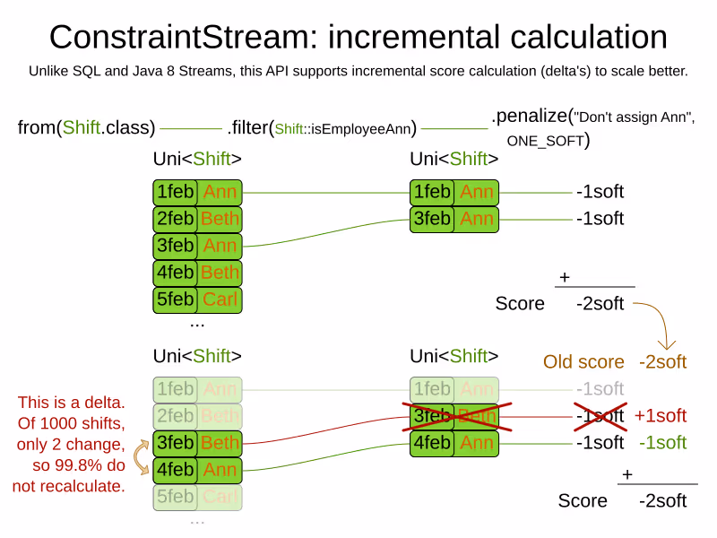
Incremental calculation

First off, unlike an EasyScoreCalculator, Constraint Streams still apply incremental score calculation to scale out, just like DRL. For example, when a move swaps the employee of two shifts, only the delta is calculated. That’s a huge scalability gain:

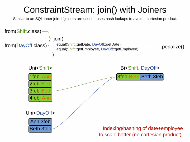
Indexing

When joining multiple types, just like an SQL JOIN operator, Constraint Streams apply hash lookups on indexes to scale better:

IDE support

Because ConstraintsStreams are written in the Java language, they piggy-back on very strong tooling support.

Code highlighting, code completion and debugging just work:

Code highlighting

DRL code in IntelliJ IDEA Ultimate:

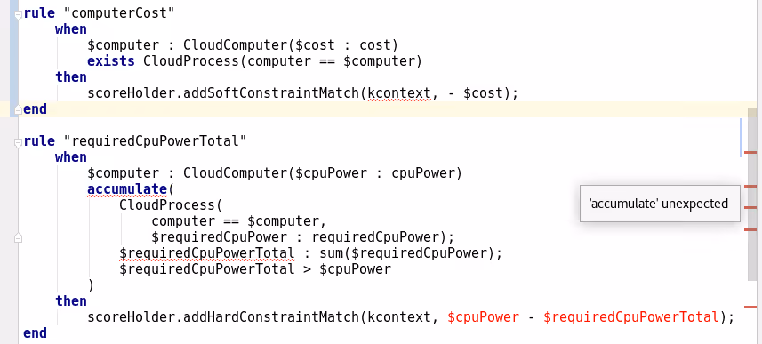
Java code using Constraint Streams in IntelliJ IDEA Ultimate, for the same constraints:

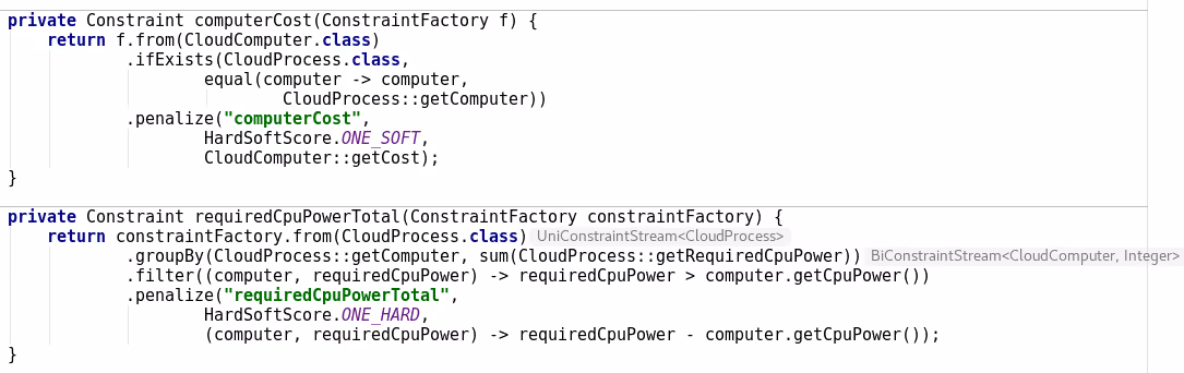
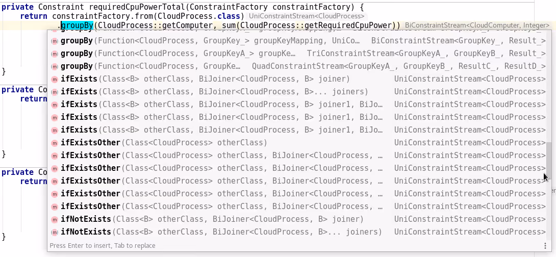
Code completion

Code completion for Constraint Streams:

Of course, all API methods have Javadocs.

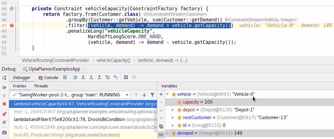
Debugging

Add a breakpoint in ConstraintStream’s filter():

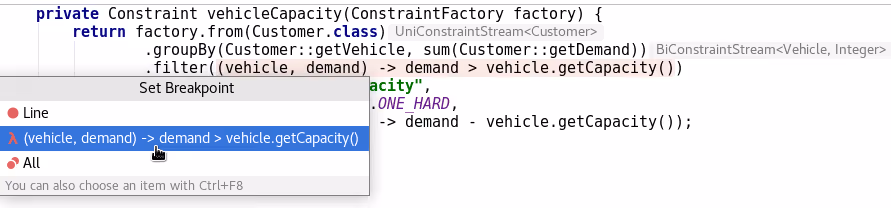
To diagnose issues while debugging:

Java syntax

Constraints written in Java with Constraint Streams follow the Java Language Specification (JLS), for good or bad. Similar logic applies when using Constraint Streams from Kotlin or Scala.

When migrating between DRL and Constraint Streams, be aware of some differences between DRL and Java:

• A DRL’s == operator translates to equals() in Java.
• Besides getters, DRL also allows MVEL expressions that translate into getters in Java.

For example, this DRL has name and ==:

rule "Don't assign Ann"
   when
       Employee(name == "Ann")
   then ...
end

But the Java variant for the exact same constraint has getName() and equals() instead:

constraintFactory.from(Employee.class)
       .filter(employee -> employee.getName().equals("Ann"))
       .penalize("Don't assign Ann", ...);

Advanced functions

The Constraint Streams API allows us to add syntactic sugar and powerful new concepts, specifically tailored to help you build complex constraints.

Just to highlight one of these, let’s take a look at the powerful groupBy method:

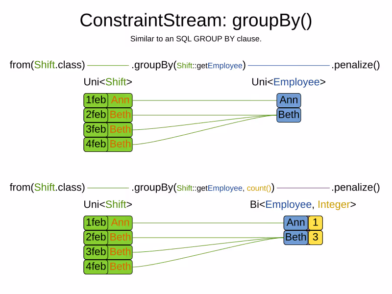
Similar to an SQL GROUP BY operator or a Java 8 Stream Collector, it supports sum(), count(), countDistinct(), min(), max(), toList() and even custom functions, again without loss of incremental score calculation.

Future work for Constraint Streams

First off, a big thanks to Lukáš Petrovický for all his work on Constraints Streams!

But this is just the beginning. We envision more advanced functions, such as load balancing/fairness methods to make such constraints easier to implement.

Right now, our first priority is to make it easier to unit test constraints in isolation. Think Test Driven Design. Stay tuned!

What is the fastest way to read a getter from a Java class without knowing the class at compilation time? Java frameworks often do this. A lot. And it can directly influence their performance. So let’s benchmark different approaches, such as reflection, method handles and code generation.

The use case

Presume we have a simple Person class with a name and an address:

public class Person {
  ...
  public String getName() {...}
  public Address getAddress() {...}
}

and we want to use frameworks such as:

• XStream, JAXB or Jackson to serialize instances to XML or JSON.
• JPA/Hibernate to store persons in a database.
• OptaPlanner to assign addresses (in case they’re tourists or homeless).

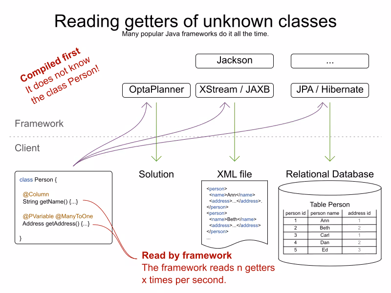
None of these frameworks know the Person class. So they can’t simply call person.getName():

  // Framework code
  public Object executeGetter(Object object) {
     // Compilation error: class Person is unknown to the framework
     return ((Person) object).getName();
  }

Instead, the code uses reflection, method handles or code generation.

But such code is called an awful lot:

• If you insert 1000 different persons in a database, JPA/Hibernate probably calls such code 2000 times:
  • 1000 calls to Person.getName()
  • another 1000 calls to Person.getAddress()
• Similarly, if you write 1000 different persons to XML or JSON, there are likely 2000 calls by XStream, JAXB or Jackson.

Obviously, when such code is called x times per second, its performance matters.

The benchmarks

Using JMH, I ran a set of micro benchmarks using OpenJDK 1.8.0_111 on Linux on a 64-bit 8-core Intel i7-4790 desktop with 32GB RAM. The JMH benchmark ran with 3 forks, 5 warmup iterations of 1 second and 20 measurement iterations of 1 second. All warmup costs are gone: increasing the length of an iteration to 5 seconds has little or no impact on the numbers reported here.

The source code of that benchmark is in this GitHub repository.

The TL;DR results

• Java Reflection is slow. (*)
• Java MethodHandles are slow too. (*)
• Generated code with javax.tools.JavaCompiler is fast. (*)
• LambdaMetafactory is pretty fast. (*)

(*) On the use cases I benchmarked with the workload I used. Your mileage may vary.

So the devil is in the details. Let’s go through the implementations, to confirm I applied typical magical tricks (such as setAccessible(true)).

Implementations

Direct access (baseline)

I’ve used a normal person.getName() call as the baseline:

public final class MyAccessor {
   public Object executeGetter(Object object) {
       return ((Person) object).getName();
   }
}

This takes about 2.6 nanoseconds per operation:

Benchmark           Mode  Cnt  Score   Error  Units
===================================================
DirectAccess        avgt   60  2.590 ± 0.014  ns/op

Direct access is naturally the fastest approach at runtime, with no bootstrap cost. But it imports Person at compilation time, so it’s unusable by every framework.

Reflection

The obvious way for a framework read that getter at runtime, without knowing it in advance, is through Java Reflection:

public final class MyAccessor {
   private final Method getterMethod;
   public MyAccessor() {
       getterMethod = Person.class.getMethod("getName");
       // Skip Java language access checking during executeGetter()
       getterMethod.setAccessible(true);
   }
   public Object executeGetter(Object bean) {
       return getterMethod.invoke(bean);
   }
}

Adding setAccessible(true) call makes these reflection calls faster, but even then it takes 5.5 nanoseconds per call.

Benchmark           Mode  Cnt  Score   Error  Units
===================================================
DirectAccess        avgt   60  2.590 ± 0.014  ns/op
Reflection          avgt   60  5.275 ± 0.053  ns/op

Reflection is 104% slower than direct access (so about twice as slow). It also takes longer to warm up.

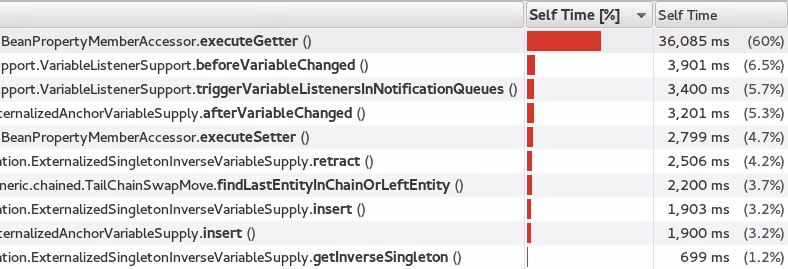
This wasn’t a big surprise to me, because when I profile (using sampling) an artificially simple Traveling Salesman Problem with 980 cities in OptaPlanner (now Timefold), the reflection cost sticks out like a sore thumb:

MethodHandles

MethodHandle was introduced in Java 7 to support invokedynamic instructions. According to the Javadoc, it’s a typed, directly executable reference to an underlying method. Sounds fast, right?

public final class MyAccessor {
   private final MethodHandle getterMethodHandle;
   public MyAccessor() {
       MethodHandles.Lookup lookup = MethodHandles.lookup();
       // findVirtual() matches signature of Person.getName()
       getterMethodHandle = lookup.findVirtual(Person.class, "getName", MethodType.methodType(String.class))
           // asType() matches signature of MyAccessor.executeGetter()
           .asType(MethodType.methodType(Object.class, Object.class));
   }
   public Object executeGetter(Object bean) {
       return getterMethodHandle.invokeExact(bean);
   }
}

Well unfortunately, MethodHandle is even slower than reflection in OpenJDK 8. It takes 6.1 nanoseconds per operation, so 136% slower than direct access.

Benchmark           Mode  Cnt  Score   Error  Units
===================================================
DirectAccess        avgt   60  2.590 ± 0.014  ns/op
Reflection          avgt   60  5.275 ± 0.053  ns/op
MethodHandle        avgt   60  6.100 ± 0.079  ns/op

Using lookup.unreflectGetter(Field) instead of lookup.findVirtual(…​) has no notable difference. I do hope that MethodHandle will become as fast as direct access in future Java versions.

Static MethodHandles (update on 2018-01-11)

I also ran a benchmark with MethodHandle in a static field. The JVM can do more magic with static fields, as explained by Aleksey Shipilёv. Aleksey and John O’Hara correctly pointed out that the original benchmark didn’t use static fields correctly, so I fixed that. Here are the amended results:

Benchmark           Mode  Cnt  Score   Error  Units
===================================================
DirectAccess        avgt   60  2.590 ± 0.014  ns/op
MethodHandle        avgt   60  6.100 ± 0.079  ns/op
StaticMethodHandle  avgt   60  2.635 ± 0.027  ns/op

Yes, a static MethodHandle is as fast as direct access, but it’s still useless, unless we want to write code like this:

public final class MyAccessors {
   private static final MethodHandle handle1; // Person.getName()
   private static final MethodHandle handle2; // Person.getAge()
   private static final MethodHandle handle3; // Company.getName()
   private static final MethodHandle handle4; // Company.getAddress()
   private static final MethodHandle handle5; // ...
   private static final MethodHandle handle6;
   private static final MethodHandle handle7;
   private static final MethodHandle handle8;
   private static final MethodHandle handle9;
   ...
   private static final MethodHandle handle1000;
}

If our framework deals with a domain class hierarchy with 4 getters, it would fill up the first 4 fields. However, if it deals with 100 domain classes with 20 getters each, totaling 2000 getters, it will crash due to a lack of static fields.

Besides, if I wrote code like this, even first year students would come tell me that I am doing it wrong. Static fields shouldn’t be used for instance variables.

Generated code with javax.tools.JavaCompiler

In Java, it’s possible to compile and run generated Java code at runtime. So with the javax.tools.JavaCompiler API, we can generate the direct access code at runtime:

public abstract class MyAccessor {
   // Just a gist of the code, the full source code is linked in a previous section
   public static MyAccessor generate() {
       final String String fullClassName = "x.y.generated.MyAccessorPerson$getName";
       final String source = "package x.y.generated;\n"
               + "public final class MyAccessorPerson$getName extends MyAccessor {\n"
               + "    public Object executeGetter(Object bean) {\n"
               + "        return ((Person) object).getName();\n"
               + "    }\n"
               + "}";
       JavaFileObject fileObject = new ...(fullClassName, source);
       JavaCompiler compiler = ToolProvider.getSystemJavaCompiler();
       ClassLoader classLoader = ...;
       JavaFileManager javaFileManager = new ...(..., classLoader)
       CompilationTask task = compiler.getTask(..., javaFileManager, ..., singletonList(fileObject));
       boolean success = task.call();
       ...
       Class compiledClass = classLoader.loadClass(fullClassName);
       return compiledClass.newInstance();
   }
   // Implemented by the generated subclass
   public abstract Object executeGetter(Object object);
}

The full source code is much longer and available in this GitHub repository. For more information on how to use javax.tools.JavaCompiler, take a look at page 2 of this article or this article. In Java 8, it requires the tools.jar on the classpath, which is there automatically in a JDK installation. In Java 9, it requires the module java.compiler in the modulepath. Also, proper care needs to be taken that it doesn’t generate a classlist.mf file in the working directory and that it uses the correct ClassLoader.

Besides javax.tools.JavaCompiler, similar approaches can use ASM or CGLIB, but those infer maven dependencies and might have different performance results.

In any case, the generated code is as fast as direct access:

Benchmark           Mode  Cnt  Score   Error  Units
===================================================
DirectAccess        avgt   60  2.590 ± 0.014  ns/op
JavaCompiler        avgt   60  2.726 ± 0.026  ns/op

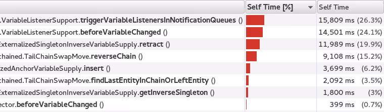
So when I ran that Traveling Salesman Problem again in OptaPlanner, this time using code generation to access planning variables, the score calculation speed was 18% faster overall. And the profiling (using sampling) looks much better too:

Note that in normal use cases, that performance gain will hardly be detectable, due to massive CPU needs of a realistically complex score calculation…​

One downside of code generation at runtime is that it infers a noticeable bootstrap cost (as discussed later), especially if the generated code isn’t compiled in bulk. So I am still hoping that some day MethodHandles will get as fast as direct access, just to avoid that bootstrap cost and the dependency pain.

LambdaMetafactory (update on 2018-01-11)

On Reddit, I received an eloquent suggestion to use LambdaMetafactory:

Getting LambdaMetafactory to work on a non-static method turned out to be challenging (due to lack of documentation and StackOverflow questions), but it does work:

public final class MyAccessor {
   private final Function getterFunction;
   public MyAccessor() {
       MethodHandles.Lookup lookup = MethodHandles.lookup();
       CallSite site = LambdaMetafactory.metafactory(lookup,
               "apply",
               MethodType.methodType(Function.class),
               MethodType.methodType(Object.class, Object.class),
               lookup.findVirtual(Person.class, "getName", MethodType.methodType(String.class)),
               MethodType.methodType(String.class, Person.class));
       getterFunction = (Function) site.getTarget().invokeExact();
   }
   public Object executeGetter(Object bean) {
       return getterFunction.apply(bean);
   }
}

And it looks good: LambdaMetafactory is almost as fast as direct access. It’s only 33% slower than direct access, so much better than reflection.

Benchmark           Mode  Cnt  Score   Error  Units
===================================================
DirectAccess        avgt   60  2.590 ± 0.014  ns/op
Reflection          avgt   60  5.275 ± 0.053  ns/op
LambdaMetafactory   avgt   60  3.453 ± 0.034  ns/op

When I ran that Traveling Salesman Problem again in OptaPlanner, this time using LambdaMetafactory to access planning variables, the score calculation speed was 9% faster overall. However, the profiling (using sampling) still shows a lot of executeGetter() time, but less than with reflection.

The metaspace cost seems to be about 2kb per lambda in a non-scientific measurement and it gets garbage collected normally.

Bootstrap cost (update on 2018-01-25)

The runtime cost matters most, as it’s not uncommon to retrieve a getter on thousands of instances per second. However, the bootstrap cost matters too, because we need to create a MyAccessor for every getter in the domain hierarchy that we want to reflect over, such as Person.getName(), Person.getAddress(), Address.getStreet(), Address.getCity(), …​

Reflection and MethodHandle have a neglectable bootstrap cost. For LambdaMetafactory it is still acceptable: my machine creates about 25k accessors per second. But for JavaCompiler it is not: my machine creates only about 200 accessors per second.

Benchmark                    Mode  Cnt        Score        Error  Units
=======================================================================
Reflection Bootstrap         avgt   60      268.510 ±     25.271  ns/op //    0.3µs/op
MethodHandle Bootstrap       avgt   60     1519.177 ±     46.644  ns/op //    1.5µs/op
JavaCompiler Bootstrap       avgt   60  4814526.314 ± 503770.574  ns/op // 4814.5µs/op
LambdaMetafactory Bootstrap  avgt   60    38904.287 ±   1330.080  ns/op //   39.9µs/op

This benchmark does not do caching or bulk complication.

Conclusion

In this investigation, reflection and (usable) MethodHandles are twice as slow as direct access in OpenJDK 8. Generated code is as fast as direct access, but it’s a pain. LambdaMetafactory is almost as fast as direct access.

Benchmark           Mode  Cnt  Score   Error  Units
===================================================
DirectAccess        avgt   60  2.590 ± 0.014  ns/op
Reflection          avgt   60  5.275 ± 0.053  ns/op // 104% slower
MethodHandle        avgt   60  6.100 ± 0.079  ns/op // 136% slower
StaticMethodHandle  avgt   60  2.635 ± 0.027  ns/op //   2% slower
JavaCompiler        avgt   60  2.726 ± 0.026  ns/op //   5% slower
LambdaMetafactory   avgt   60  3.453 ± 0.034  ns/op //  33% slower

Your mileage may vary.

So we solved the planning problem and found a best solution which has a score of 0hard/-123soft. Why -123soft? Where does that penalty come from? Which constraints are broken? Let’s see how we can break down the score and visualize the pain points in a UI.

Let’s approach this problem from two sides on the course scheduling example:

Break down score per constraint type

In the top-down approach, we split up the score per constraint type (so per score rule):

Constraint typeScore impactRoom capacity-100softRoom stability-40softCurriculum compactness-3softTotal-123soft

The room capacity constraint is broken the most: it causes for 81% (100/123) of the score loss. Maybe the school should invest in more classrooms?

Heat map with score impact per planning entity

In the bottom-up approach, we visualize the score impact per lecture:

• Red lectures impact hard constraints.
• Orange lectures impact only soft constraints. The higher the impact, the heavier the color.
• White lectures don’t impact the score.

As OptaPlanner, now continued as Timefold Solver, finds better and better solutions, there is less and less orange on the heat map. Looks like the history courses are particularly hard to schedule. Maybe the school should look for an additional history teacher?

(*) Notice that -1soft is shared by multiple lectures: 3 lectures break the room stability constraint together because two of them use a different room than the other one.

Show me the API

OptaPlanner 7 provides this information out of the box through the ConstraintMatch API:

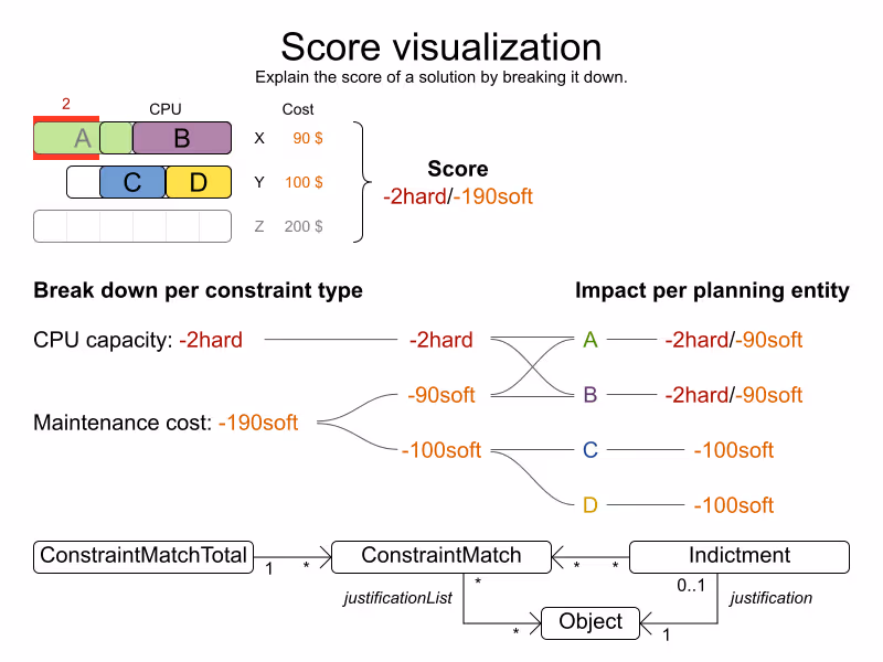
First build a ScoreDirector with Solver.getScoreDirectorFactory() and then:

• Break down the score per constraint type with ScoreDirector.getConstraintMatchTotals(). Each ConstraintMatchTotal represents one score rule and has its total score.
• Determine the score impact per planning entity with ScoreDirector.getIndictmentMap(). Each Indictment holds the total score impact of one planning entity. Use that score to create the heat map in your UI.

Conclusion

Help the user make sense of the resulting score. Visualize which constraints and planning entities cause most harm.

Planned, planning education for real world stuff

When you put your optimization project into production, your enterprise will decrease expenses, increase customer satisfaction, improve employee happiness and/or reduce its ecological footprint. But if the end-users reject your implementation, none of that will happen. Let’s take a look why they might do that.

There are 7 common ways to fail your optimization project:

1. Ignore the user’s plan
2. Neglect a hard constraint
3. Decide all score weights up front
4. Change tentative plans drastically
5. Presume there is always a feasible plan
6. Average out fairness or load balancing
7. Focus on only 1 stakeholder

Let’s take a look at each one in detail and the 7 ways to make your project a success:

1. Keep the user in control

Initially, nobody trusts a new system that takes input (the planning problem) and produces output (the solution) through a non-obvious transformation. To build this trust, allow the user to override OptaPlanner’s choices.

For example in Cloud Balancing, if the user locks the green process to computer Y, the planning engine must respect that:

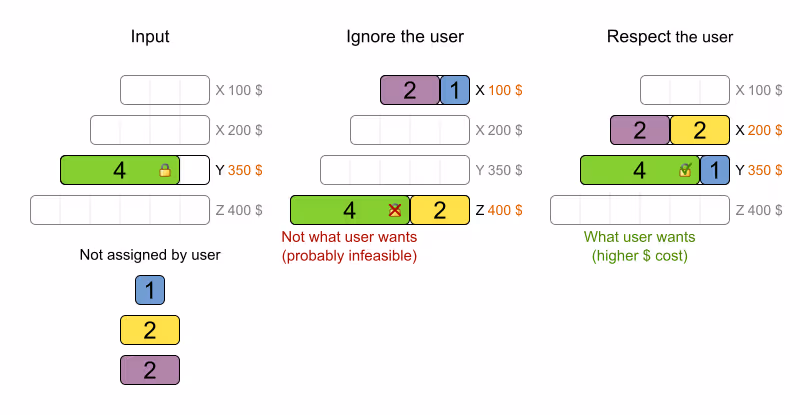
It’s not an all-or-nothing situation: the user and OptaPlanner (now continued as Timefold) work together (and the user is in charge). For a detailed use case, see this blog with video.

Technically, this is implemented through immovable planning entities: a simple boolean method that checks if the process is pinned.

2. Implement all hard constraints

An optimal solution that takes only 99% of the hard constraints into account is 100% useless. So implement all hard constraints.

For example in Vehicle Routing, let’s suppose we need to pickup nuclear cargo too, but forget to add a hard constraint to pick those up with a special vehicle:

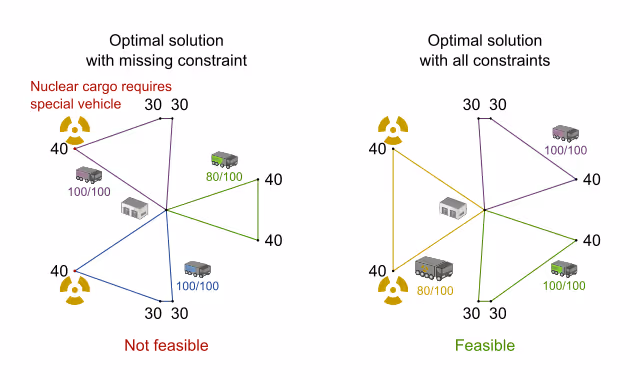
As you can see, taking that extra hard constraint into account can change the optimal solution entirely.

Technically, OptaPlanner supports any type of constraint: unlike other solvers, it doesn’t care if the constraint is linear, quadratic or worse. As long as it can compare the score of any 2 solutions, it finds the best one. That enables you to implement all constraints: none will be out of reach.

3. Don’t hard-code the score weights

Most business people can’t tell us the best score weights until they’ve seen the impact of those weights on their schedule. So allow the user to change the score weights at runtime and quickly see the effect of his/her changes on the solution.

For example in Cloud Balancing: should we focus on load balancing or on cost reduction?

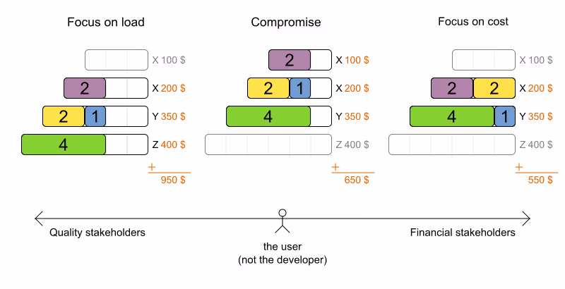
Some constraints work together, others work against each other. Especially for that last kind (as shown above), different stakeholders within the same enterprise can disagree on the score weights. Empower the project owner to settle those negotiations by directly changing the weights in the UI.

Technically, simply add a singleton with the score weights in the dataset and use those weights in the constraints. Look for a *ConstraintConfiguration class in some of the OptaPlanner examples.

4. Avoid disruption when replanning

At some point, a plan becomes tentative or even final. Any changes after that point can be very disruptive to anyone involved in that plan. But ad hoc changes, such as an employee calling in sick or malfunctioning equipment, will make your plan infeasible and force you to replan it.

For example in Cloud Balancing, a computer might break down:

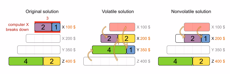
The middle solution is slightly more cost-effective, but the last solution is far less disruptive. Especially when scheduling people, who planned their social life based on the tentative schedule, it’s important to minimize disruption.

Technically, we penalize the number of processes that moved, by keeping track of the old tentative computer assignment for each process too.

Another way to make this easier is to also do backup planning. For example in employee rostering, we assign 3 reserve shifts as backups to 3 employees: if another employee calls in sick, one of the reserve employees takes over automatically, without replanning. Only when more than 3 employees call in sick, we actually need to do (non disruptive) replanning.

5. Account for overconstrained planning

It can happen that there aren’t enough resources to solve a planning problem without breaking a hard constraint. In that case, instead of delivering an infeasible plan, it’s often better to leave some entities unassigned (as little as possible of course).

For example in employee rostering, when we need to assign 4 late shifts on the same day and we only have 3 employees, it’s better to leave 1 shift unassigned than to assign an employee to 2 shifts at the same time.

Going one step further, we can add virtual resources to indicate how many extra resources to buy/hire. For example in the same employee rostering case, we could add 2 virtual employees. After solving, it will use one of these which tell us that we can make the schedule feasible again by hiring 1 extra employee.

Technically, we need to treat unassigned (or virtual assigned) entities differently in the constraints and add a medium score level (between hard and soft) to penalize the number of unassigned (or virtual assigned) entities.

6. Be fair (load balancing)

When distributing work across humans (or machines), don’t use averages. Instead, the worst off human (or machine) counts the most.

For example in employee rostering we want to distribute the shifts evenly, but we can’t make it perfectly fair due to skill and other hard constraints. It’s not about minimizing overtime on average, but about minimizing overtime of the worst off employee:

In the last solution, more employees are happy, but the worst employee is worse off, so it’s less fair than the middle solution.

Technically: penalize the square of the number of shifts per employee.

7. Create a win-win for all stakeholders

In a big organization, many different groups will want to tune the constraint weights in their favor. For example: management will often want to maximize cost reduction, but unions will want to maximize employee happiness and job security. Whenever possible, aim for a solution that improves the status quo for all stakeholders. They can always negotiate the tuning of the score weights later.

In a war story that came to my ear, I’ve heard about a VRP case for inspectors that heavily reduced driving time to inspection sites, allowing the same work to be done in less time. Because the prototype focused only on using fewer inspectors, the unions shot it down. If instead the prototype had focused on increasing inspection time, it would have increased inspection quality, reduced worker stress, lowered fuel expenses and decreased the need for new hires. That’s far more acceptable to all stakeholders.

Conclusion

Project success doesn’t depend on solution quality alone. There are a lot of factors that can make or break a project. In this article I highlighted some of the more social ones. Luckily, you can handle these additional requirements with OptaPlanner (now continued as Timefold) too. Don’t let them catch you off guard!

Are we smarter than machines when it comes to planning? Or can automated planning beat humans? I did an experiment with a group of innocent software engineers. These are the results.

Methodology

During my last 2 deep dive trainings, I asked the attendees to manually solve a simple planning problem, to introduce them to the difficulty of planning optimization.

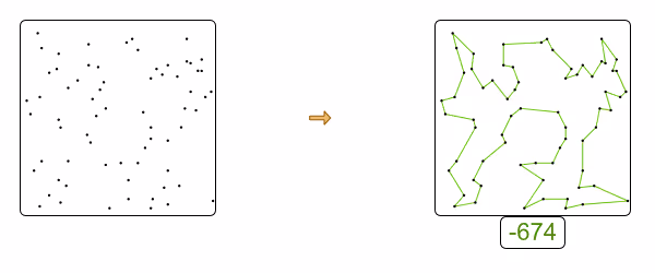
I gave them a Traveling Salesman Problem (TSP) and asked them to connect the dots to find the shortest tour possible:

They laughed. Isn’t this a kids game? Yes, except that the dots are not numbered and you’re not looking for Mickey Mouse.

Calculating a trip’s distance on paper is not practical, so they recreated their trips in the TSP example in OptaPlanner examples (only since 6.3.0.Beta1) to calculate the distance automatically. You can try this assignment yourself: right-click in the example’s UI to manually create a trip.

Their first attempt and their best attempt in a time window of almost 30 minutes was recorded. This is the optimal solution that we hoped to find:

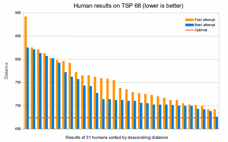
Results

No one found the optimal solution. Most people didn’t even find a near optimal solution (including me):

First attemptBest attemptOptimal674674Average human752732Average human worse than optimal12%9%

On average, a human’s best result was 9% worse than the optimal solution. That means it roughly takes 9% more time and 9% more fuel to visit those locations. That’s expensive.

That’s just on a small problem with only 1 constraint! In the real world, other constraints need to be taken into account, such as vehicle capacity, real road networks and custom business constraints. All of these make it harder.

Below are the individual results:

First attemptBest attempt825825821821813813892807802802792792772772762762798757765743758742727727765714755714712712712712729710759710723706705705796702738702702702720701725700717699699699701693692692735688692676

The best attempt of the best human was only 0.3% worse than optimal. That’s a very nice result. If I recall correctly, he did take longer than 30 minutes to find it. Was this skill or luck (or a combination of both)? The second best human (out of 31 people) was 2% worse than optimal.

With automated planning, such as OptaPlanner (now continued as Timefold Solver), we can beat the human results, in far less time. We can also scale to bigger datasets with more constraints. Does this mean we can get rid of the human planner?

Do we need a human planner?

We still need a human planner: not to search for the best plan, but to define what to search for. A search engine like Google can search the web, but it needs to be told what to look for. Similarly, any automated solver (including Timefold Solver) can optimize a planning, but it needs to be told what to optimize for.

In a non-trivial enterprise, defining what the business wants/needs to optimize, is not a simple task. It involves talking to the business departments and iteratively tweaking those constraints. We still need a human to that. And as the business changes (market changes, labor regulations changes, …​) those constraints will change too. Again, we need a human to watch over the planner. We also need someone to input the data and validate the results. Furthermore, the human needs to stay in control.

But ask yourself: Who of these 2 contenders will win a knowledge quiz?

• The smartest person on the planet
• An average graduate with internet and Wikipedia access

Similarly, who do you want to optimize the planning in your organization? Someone with or without automated planning assistance?

Earlier this week, The Washington Post published an article about how a data genius has computed the ultimate American road trip. The only problem…​ it contains several mistakes! It’s not the optimal route, nor the shortest route, nor the fastest route. Let’s take a look at the problems and how we can fix each of them.

The goal

The Ultimate American Road Trip stops at 50 national natural landmarks, national historic sites and national monuments in the US. The goal is to find the fastest trip to visit all of these locations. This is known as a Traveling Salesman Problem.

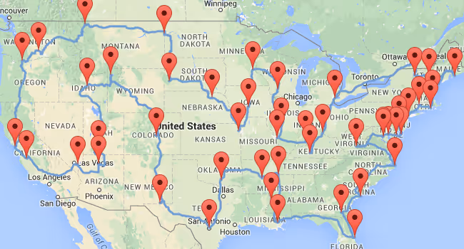
The original solution (Olson’s algorithm)

Here’s the original solution based on Randy Olson’s blog shown with Google Maps:

Note that I had to recreate the datasets. I’ve used exact latitude longitude coordinates (instead of location names) to avoid ambiguity and get more accurate routes.

The Washington Post even claims that the trip above is the fastest trip (Olson’s blog doesn’t make this claim), but it’s not:

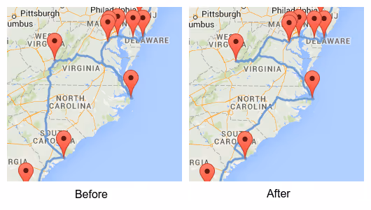
Bug 1: Better optimization algorithms give better results

A few days ago, William J. Cook already proved with Concorde that there’s a shortest and faster path near Iowa. With OptaPlanner (now continued as Timefold Solver) I come to the same conclusion:

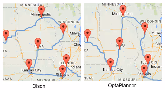
This reduces the total time by 1h 35m 40s and the total distance by 34km 515m.

Bug 2: Ghost driving (driving on the wrong side of the road) is illegal

Road distances are not symmetric. Driving from A to B is not the same as driving from B to A (if you adhere to traffic rules, of course):

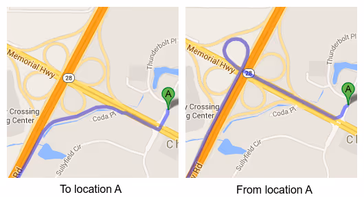
If we take this into account, the fastest path near Carolina changes:

On the left is the path found by both Olson and Cook (and by myself when using Olson’s symmetrical distances). On the right is my path, which reduces the total time by another 49m 36s (if both paths are computed using asymmetric distances), but increases the distance by 805m.

Bug 3: Google Maps does not return the shortest routes

Do we want the shortest or the fastest trip? We used Google Maps to calculate the fastest route between every pair of locations. So if we’re aiming for the fastest trip, that’s fine.

However, if we’re aiming for the shortest trip, then we should be asking Google Maps for the shortest routes, which can be drastically different:

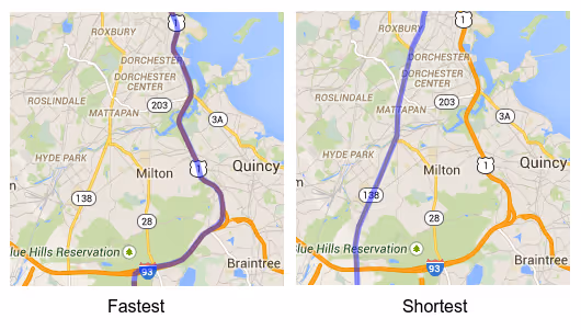
Contrary to popular belief, the shortest trip on the fastest routes is not the shortest trip.

Most people tend to prefer highways over dirt roads, so they prefer the fastest trip over the shortest trip. In more advanced use cases, we would also want to take additional constraints into account:

• Not all routes are equally beautiful or equally safe.
• Consider optional places to visit, as long as they don’t impact the length of our trip too much.
• Consider time constraints: to see that sunset at the ocean, we’ll need to arrive there before the evening.

That’s when a customizable solver such as Timefold Solver becomes really useful.

Conclusion

By using better algorithms and a more accurate model (without ghost driving), our trip is 2h 25m 16s faster:

DatasetTimeTotal time gainDistanceTotal distance gainOlson (Clockwise)232h 43m 10s 22'602km 201m Iowa fix (Clockwise)231h 7m 30s1h 35m 40s22'567km 686m34km 515mIowa and Carolina fix (Clockwise)230h 17m 54s (best)2h 25m 16s22'568km 491m33km 710m

Interestingly enough, if we’re looking for the shortest trip (and we ignore bug 3 because we prefer highways), we notice that the same trip (with both fixes) in the reverse direction is the shortest:

DatasetTimeTotal time gainDistanceTotal distance gainOlson (Counterclockwise)232h 46m 58s 22'612km 070m Iowa fix (Counterclockwise)231h 16m 52s1h 30m 06s22'562km 668m49km 402mIowa and Carolina fix (Counterclockwise)230h 27m 26s2h 19m 32s22'560km 688m (best)51km 382m

This is my solution to the Ultimate American Road Trip (with those fixes):

Drive it clockwise to optimize time!

After OptaPlanner (now Timefold) finds the best solution for a Vehicle Routing Problem, users usually want to see it on a real map, such as Google Maps or OpenStreetMap. The optaplanner-webexamples.war for OptaPlanner 6.3 now demonstrates that.

Visualization

In the case below, I’ve solved a VRP problem with 50 locations and 8 vehicles and projected the best solution with Leaflet and Google Maps. It’s a case of capacitated vehicle routing: each vehicle can carry 100 items and each location needs a number of items picked up.

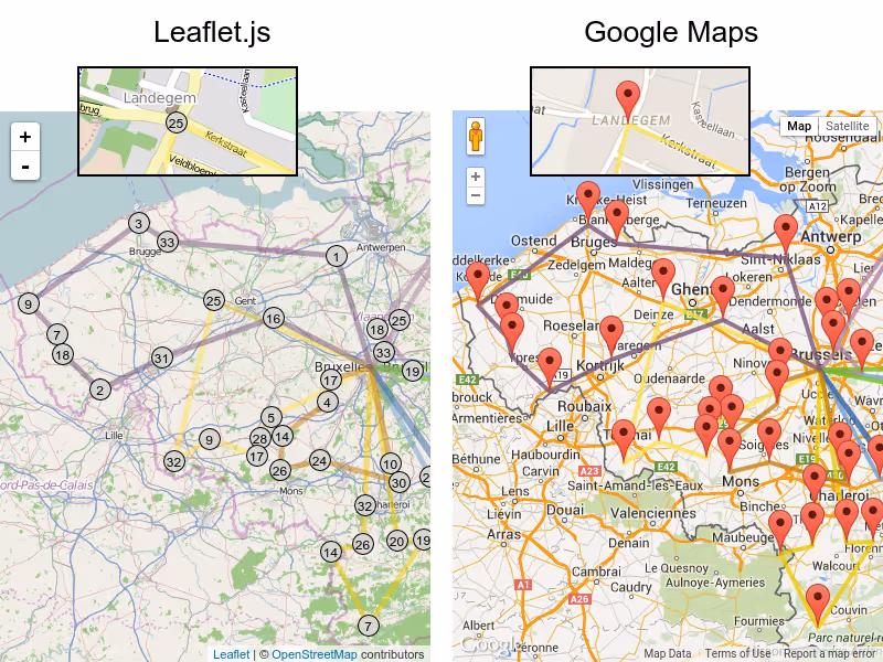
Despite that the lines are shown as straight between locations, actual road distances were used in the optimization calculations. In total, the vehicles drive a little under 32 hours, so on average 4 hours per vehicle (includes location service time). This solution doesn’t take into account rush hour yet, but if such traffic prediction data were available, we can make OptaPlanner apply that too, which could result in a different best solution.

In the web UI, we can zoom in on a specific location, such as the Landegem town center, where we need to pickup 25 items. In this solution, those items are picked up by the yellow vehicle.

The visualization was implemented in 2 different ways:

Leaflet.js

Leaflet.js is an open source JavaScript that uses OpenStreetMap data.

Google Maps

Google Maps is a proprietary JavaScript that uses Google data.

Apply it now in your case

If you’re using the latest OptaPlanner final release (6.2.0.Final at the time of writing), you easily do such visualization too: those webexamples don’t require any APIs new in optaplanner-core 6.3, so download the nightly snapshot and look for webexamples/sources to see how it’s done.

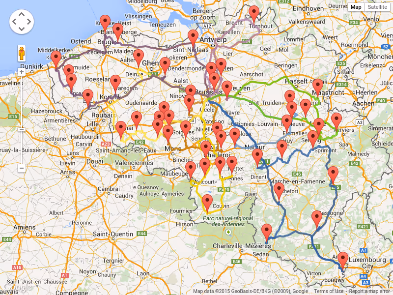
Update

With Google Map Directions we can also visualize the actual roads used:

What’s the cost of trace/debug logging in production? What’s the performance cost of logging to a file? In these benchmarks, I compare the performance impact of logging levels (error, warn, info, debug, trace) and logging appenders (console appender, file appender) on several realistic OptaPlanner use cases.

Benchmark methodology

• Logging implementation: SFL4J 1.7.2 with Logback 1.0.9 (Logback is the spiritual successor of Log4J 1)
• Logging configuration (logback.xml):

<?xml version="1.0" encoding="UTF-8"?>
<configuration>

 <appender name="appender" class="ch.qos.logback.core.ConsoleAppender">
   <encoder>
     <pattern>%d [%t] %-5p %m%n</pattern>
   </encoder>
 </appender>

 <logger name="org.optaplanner" level="info"/>

 <root level="warn">
   <appender-ref ref="appender"/>
 </root>

</configuration>

Which results in output like this:

2015-02-23 08:07:35,310 [main] INFO  Solving started: time spent (18), best score (uninitialized/0hard/0soft), environment mode (REPRODUCIBLE), random (JDK with seed 0). 2015-02-23 08:07:35,363 [main] INFO  Construction Heuristic phase (0) ended: step total (6), time spent (71), best score (0hard/-5460soft). 2015-02-23 08:07:35,641 [main] INFO  Local Search phase (1) ended: step total (1), time spent (349), best score (0hard/-5460soft). 2015-02-23 08:07:35,652 [main] INFO  Solving ended: time spent (360), best score (0hard/-5460soft), average calculate count per second (905), phase total (2), environment mode (REPRODUCIBLE).

• VM arguments: -Xmx1536M -server
  Software: Linux 3.2.0-59-generic-pae
  Hardware: Intel® Xeon® CPU W3550 @ 3.07GHz
• Each run solves 13 planning problems with OptaPlanner. Each planning problem runs for 5 minutes. It starts with a 30 second JVM warm up which is discarded.
• Solving a planning problem involves no IO (except a few milliseconds during startup to load the input). A single CPU is completely saturated. It constantly creates many short-lived objects, and the GC collects them afterwards.
• The benchmarks measure the number of scores that can be calculated per millisecond. Higher is better. Calculating a score for a proposed planning solution is non-trivial: it involves many calculations, including checking for conflicts between every entity and every other entity.

Logging levels: error, warn, info, debug and trace

I ran the same benchmark set several times with a different OptaPlanner logging level:

 <logger name="org.optaplanner" level="error|warn|info|debug|trace"/>

All other libraries (including Drools) were set to warn logging. The logging verbosity of OptaPlanner differs greatly per level:

• error and warn: 0 lines
• info: 4 lines per benchmark, so less than 1 line per minute.
• debug: 1 line per step, so about 1 line per second for Tabu Search and more for Late Acceptance
• trace: 1 line per move, so between 1k and 120k lines per second

These are the raw benchmark numbers, measured in average score calculation count per second (higher is better):

Logging levelCloud balancing 200cCloud balancing 800cMachine reassignment B1Machine reassignment B10Course scheduling c7Course scheduling c8Exam scheduling s2Exam scheduling s3Nurse rostering m1Nurse rostering mh1Sport scheduling nl14Error66065618661192303275962828370103307121400137181248Warn66943621911226783268862978303105177182394236601278Info67393631921237343246161888299103307108394436541252Debug60254559381189173273560548062103107104390435861244Trace251592521440346206295585734792296642336031381156Dataset scale120k1920k500k250000k217k145k1705k1613k18k12k4kAlgorithmLate AcceptanceLate AcceptanceTabu SearchTabu SearchLate AcceptanceLate AcceptanceTabu SearchTabu SearchTabu SearchTabu SearchTabu Search

I’ll ignore the difference between error, warn and info logging: The difference is at most 4%, the runs are 100% reproducible and I didn’t otherwise use the computer during the benchmarking, so I presume the difference can be blamed on the JIT hotspot compiling or CPU luck.

What does turning on Debug or Trace logging cost us in performance (versus Info logging)?

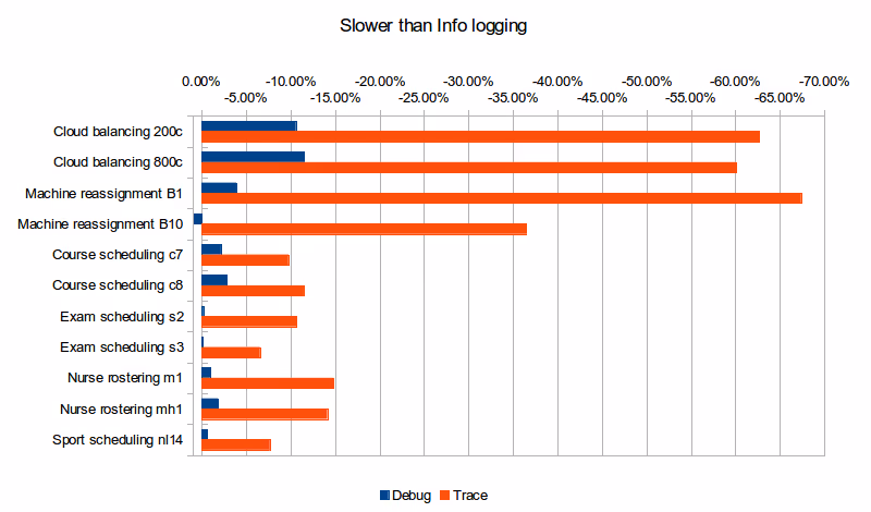
Logging levelCloud balancing 200cCloud balancing 800cMachine reassignment B1Machine reassignment B10Course scheduling c7Course scheduling c8Exam scheduling s2Exam scheduling s3Nurse rostering m1Nurse rostering mh1Sport scheduling nl14Debug-10.59%-11.48%-3.89%0.84%-2.17%-2.86%-0.19%-0.06%-1.01%-1.86%-0.64%Trace-62.67%-60.10%-67.39%-36.45%-9.74%-11.47%-10.66%-6.56%-14.81%-14.12%-7.67%Dataset scale120k1920k500k250000k217k145k1705k1613k18k12k4kAlgorithmLate AcceptanceLate AcceptanceTabu SearchTabu SearchLate AcceptanceLate AcceptanceTabu SearchTabu SearchTabu SearchTabu SearchTabu Search

Trace logging is up to almost 4 times slower! The impact of Debug logging is far less, but still clearly noticeable in many cases. The use cases that use Late Acceptance (Cloud balancing and Course scheduling), which therefore do more debug logging, seem to have a higher performance loss (although that might be in the eye of the beholder).

But wait a second! Those benchmarks use a console appender. What if they use a file appender, like in production?

Logging appenders: appending to the console or a file

On a production server, appending to the console often means losing the log information as it gets piped into /dev/null. Also during development, the IDE’s console buffer can overflow, causing the loss of log lines. One way to avoid these issues is to configure a file appender. To conserve disk space, I used a rolling file appender which compresses old log files in zip files of 5MB:

 <appender name="appender" class="ch.qos.logback.core.rolling.RollingFileAppender">
   <file>local/log/optaplanner.log</file>
   <rollingPolicy class="ch.qos.logback.core.rolling.FixedWindowRollingPolicy">
     <fileNamePattern>local/log/optaplanner.%i.log.zip</fileNamePattern>
     <minIndex>1</minIndex>
     <maxIndex>3</maxIndex>
   </rollingPolicy>
   <triggeringPolicy class="ch.qos.logback.core.rolling.SizeBasedTriggeringPolicy">
     <maxFileSize>5MB</maxFileSize>
   </triggeringPolicy>
   <encoder>
     <pattern>%d [%t] %-5p %m%n</pattern>
   </encoder>
 </appender>

These are the raw benchmark numbers, measured again in average score calculation count per second (higher is better):

Logging appender and levelCloud balancing 200cCloud balancing 800cMachine reassignment B1Machine reassignment B10Course scheduling c7Course scheduling c8Exam scheduling s2Exam scheduling s3Nurse rostering m1Nurse rostering mh1Sport scheduling nl14Console Info67393631921237343246161888299103307108394436541252File Info66497630651237583319563028338104677238402237061256Console Debug60254559381189173273560548062103107104390435861244File Debug55248522611221443122062238241104827118394535891238Console Trace251592521440346206295585734792296642336031381156File Trace10162107081252895554416516767645532278926781101

What does file appender cost us in performance (versus console appender)?

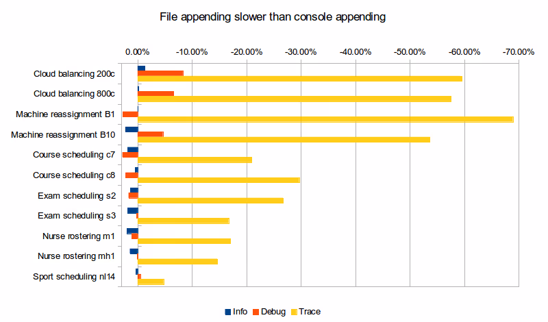
Logging levelCloud balancing 200cCloud balancing 800cMachine reassignment B1Machine reassignment B10Course scheduling c7Course scheduling c8Exam scheduling s2Exam scheduling s3Nurse rostering m1Nurse rostering mh1Sport scheduling nl14Info-1.33%-0.20%0.02%2.26%1.84%0.47%1.33%1.83%1.98%1.42%0.32%Debug-8.31%-6.57%2.71%-4.63%2.79%2.22%1.67%0.20%1.05%0.08%-0.48%Trace-59.61%-57.53%-68.95%-53.68%-20.93%-29.67%-26.71%-16.71%-16.99%-14.66%-4.76%

For info logging, it doesn’t really matter. For debug logging, there’s a noticeable slowdown for a minority of the cases. Trace logging is an extra up to almost 4 times slower! And it stacks with our previous observation: In the worst case (Machine reassignment B1), trace logging to a file is 90% slower than info logging to the console.

Conclusion

Like all diagnostic information, logging comes at a performance cost. Good libraries carefully select the logging level of each statement to balance out diagnostic needs, verbosity and performance impact.

Here’s my recommendation for OptaPlanner users: In development, use debug (or trace) logging with a console appender by default, so you can see what’s going on. In production, use warn (or info) logging with a file appender by default, so you retain important information.

‍