Blog
Technician scheduling software in 2027: Essential capabilities for modern field service
What should technician scheduling software actually do? Nine essential capabilities, from skill matching and SLA priorities to real-time replanning, explainability, and API integration.
Technician scheduling software assigns field technicians to jobs and plans their days so that the right person, with the right skills, arrives within the promised window without wasting hours on the road.
The best tools do this automatically across hundreds or thousands of technicians, and they keep the plan valid as the day changes.
Most products in this category show a calendar and a map. The difference between them is what happens underneath: whether the software can weigh skills, time windows, SLAs, travel, and working-hour rules together, or whether it leaves those tradeoffs to a dispatcher.
This guide lists nine capabilities that separate modern technician scheduling from a digital whiteboard. It's written for operations leaders comparing tools and for product teams at field service software companies deciding what their own scheduling engine needs.
Why technician scheduling has become harder
Two pressures are pushing field service teams to rethink how they schedule.
- The first is labor. In the US HVAC trade alone, industry estimates put the technician shortage at around 110,000 open positions. When every skilled technician counts, a schedule that wastes an hour of their day on avoidable driving is a real capacity problem.
- The second is expectations. Customers expect narrow arrival windows, live updates, and a fix on the first visit. Nobody wants to be anticipating their technician coming in all day.
Both pressures land on the schedule.
Nine essential capabilities
1. Skill and certification matching
The software should know what each job requires and what each technician can do, including certifications, seniority, languages, and equipment access. Hard requirements (a gas-safe certificate) should never be violated. Softer preferences (a technician the customer has worked with before) should be encouraged but not forced.
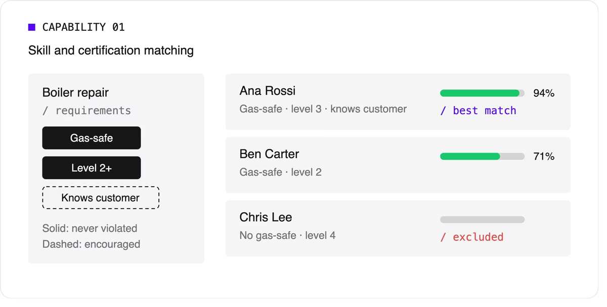
Look for support for skill levels and customer affinity in addition to simple yes-or-no skills. Matching the right skills is also one of the most direct ways to improve first-time fix rates.
2. Time windows and SLA priorities
Jobs come with customer availability windows, and many come with contractual deadlines.
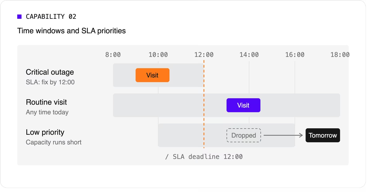
The software needs to treat a critical SLA differently from a routine visit that can move to tomorrow. That means supporting multiple time windows per job, priority levels, and deadlines that can push lower-priority work out of the plan when capacity runs short.
3. Travel-aware planning with real road data
A schedule that assumes straight-line distances will fall apart on the road. Technician scheduling software should use real travel times, ideally with support for traffic patterns and your own map provider if you already have one.
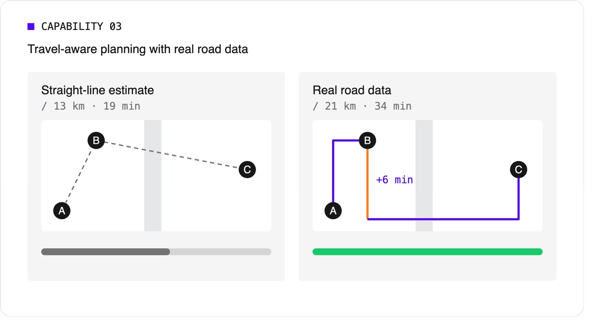
It should let you choose what to minimize, total travel time or total distance, because the two goals give different answers.
4. Multi-technician visits and job dependencies
Some jobs need two or more people on site at the same time for safety or lifting. Others must happen in order, sometimes with a delay: isolate the power before rewiring, or let a surface dry before painting.
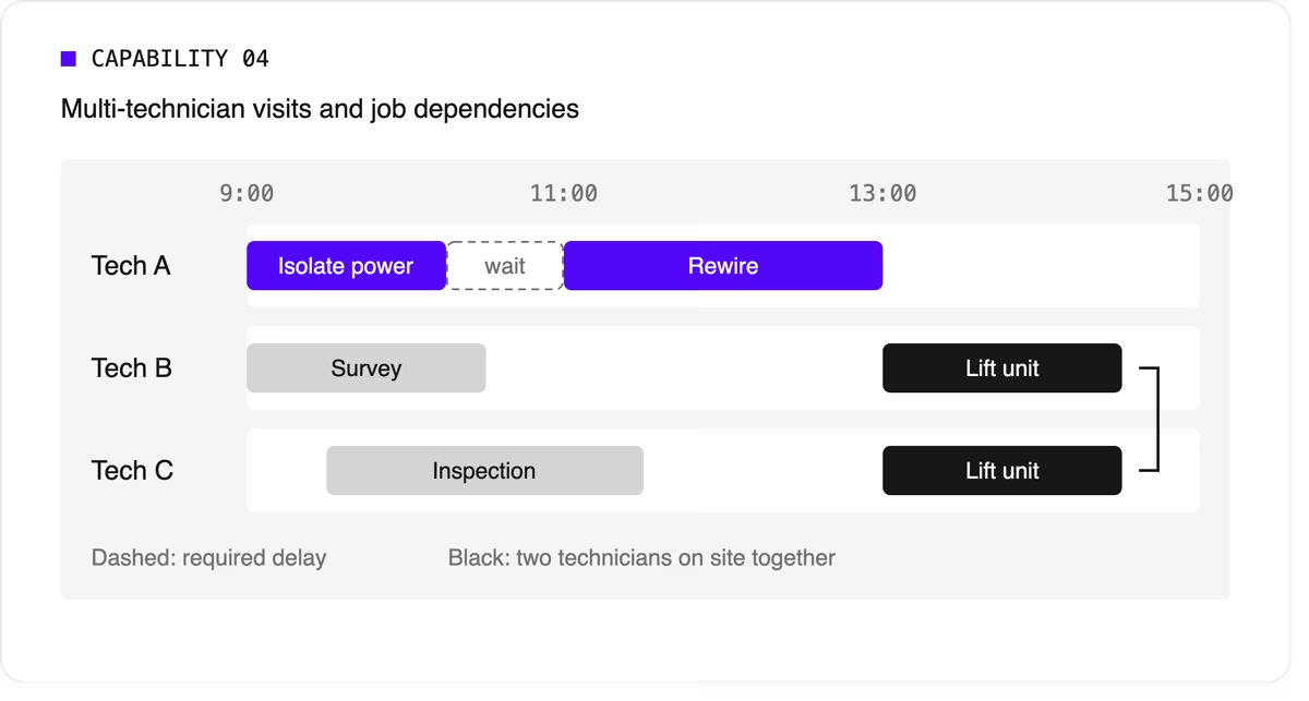
Many tools can't express these rules, so dispatchers track them by hand. If your operation has them, this capability is non-negotiable.
5. Working hours, breaks, and fairness
The plan has to respect shift start and end times, mandatory breaks, maximum working hours, and overtime rules. It should also spread work fairly so the same technicians don't always get the long days or the difficult jobs. Fairness affects retention, and retention matters more when technicians are hard to replace.
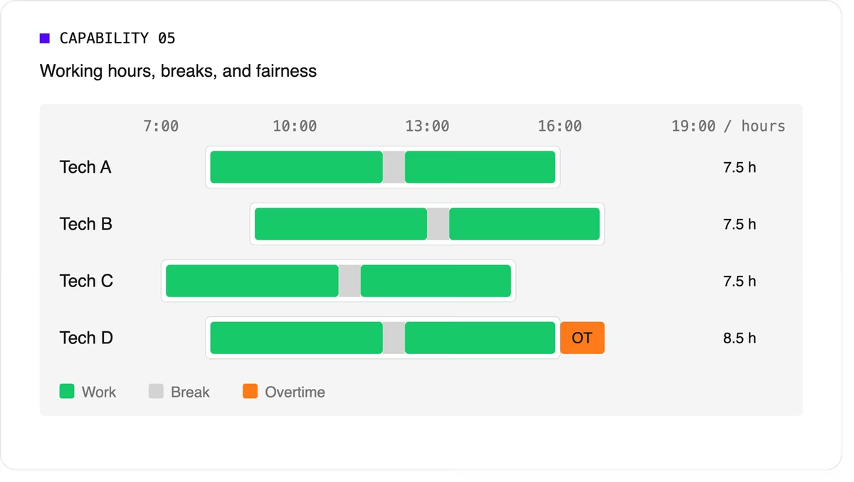
Scheduling software can support labor-law-style rules as constraints, but your organization remains responsible for verifying compliance with the regulations that apply to you.
6. Real-time replanning
Every schedule meets reality by mid-morning. A technician calls in sick, a job overruns, or an urgent call comes in. The software should replan quickly while changing as little as possible for everyone else. It should also let dispatchers lock (pin) jobs that are already in progress or confirmed with the customer.
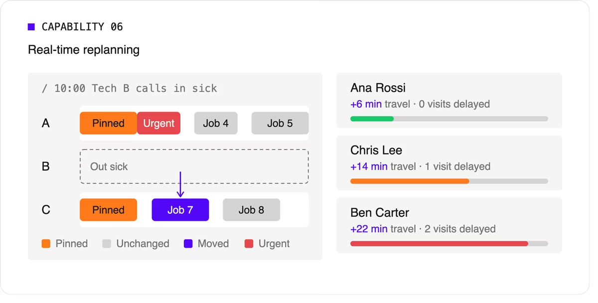
A strong version of this capability also recommends options. When a new urgent job arrives, the dispatcher should see which technicians could take it and what each choice would cost in travel or delayed work.
7. Explainability
Dispatchers and managers won't trust a plan they can't understand. Good technician scheduling software shows why a job was assigned the way it was, which rules were bent, and why some jobs couldn't be scheduled at all.
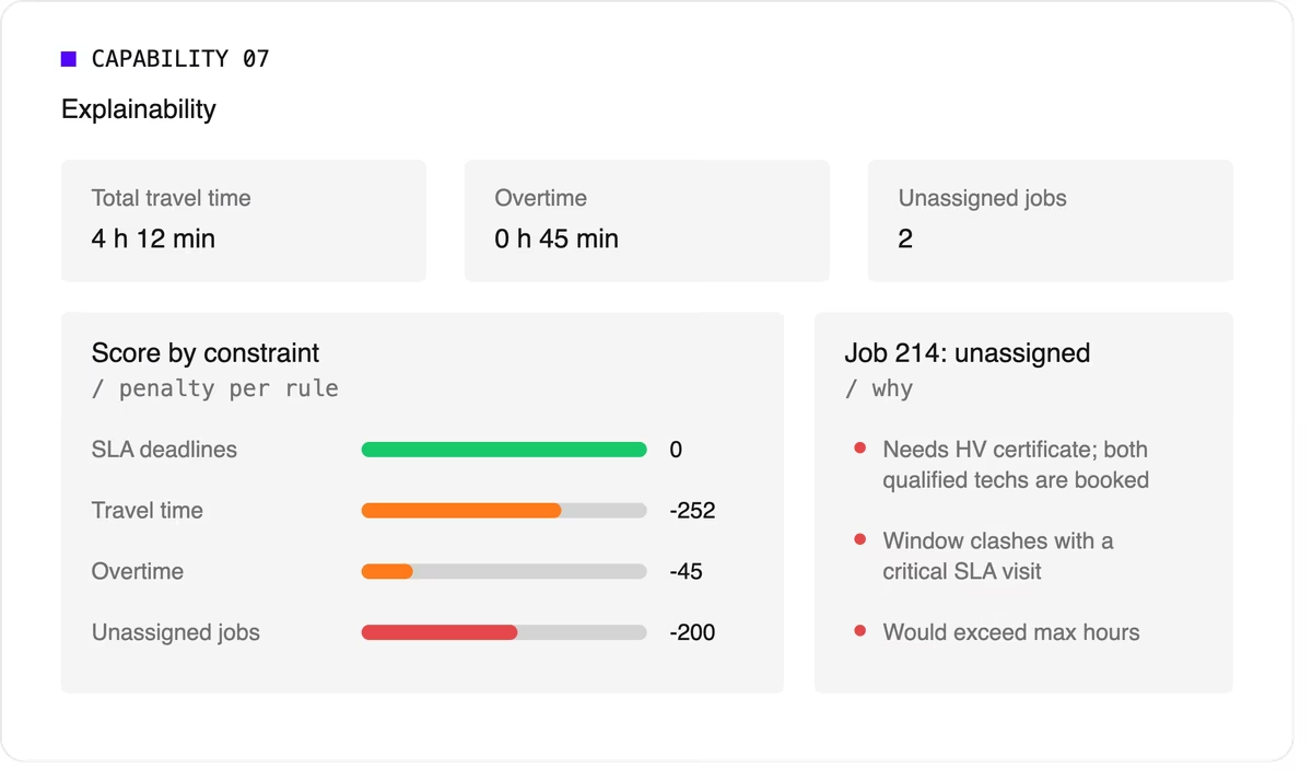
Look for a breakdown by constraint and clear metrics such as total travel time, overtime, and unassigned jobs.
8. Configurable priorities
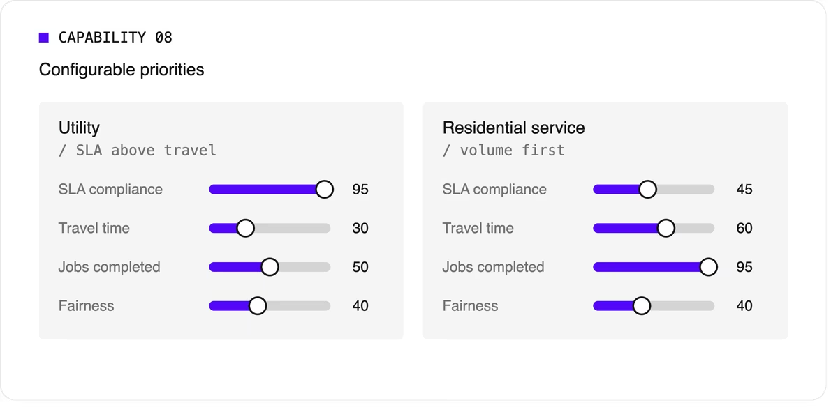
Every operation weighs its goals differently. A utility may put SLA compliance far above travel savings, while a residential service company may care most about completing as many jobs as possible per day. The software should let you adjust the relative weight of each goal without rewriting the underlying logic.
9. Integration and scale
Scheduling doesn't live on its own. It needs job data from your FSM or work order system, technician data from HR or workforce tools, and a way to push the finished plan to mobile apps. An API-first design makes this far easier than a closed tool with a separate interface.
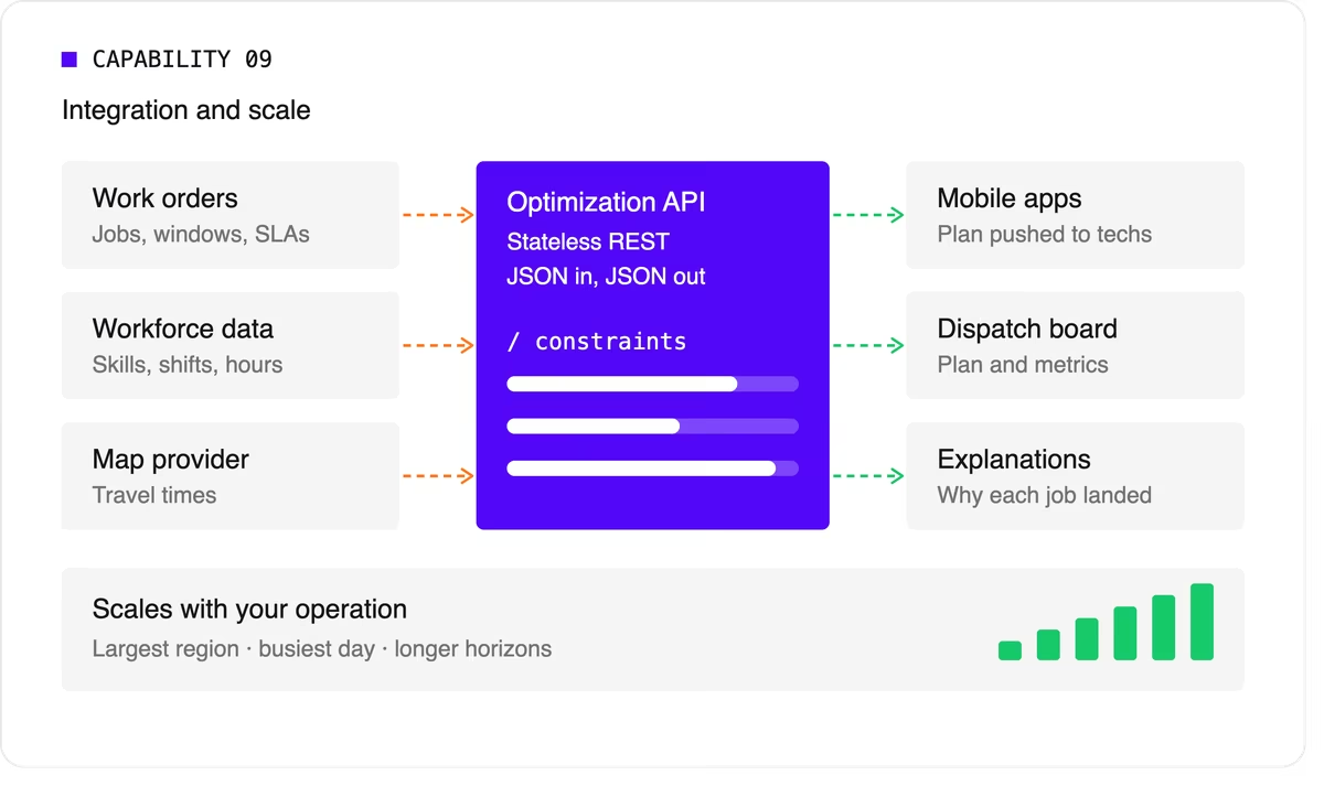
Scale matters too. The software should handle your largest region on your busiest day, and it should keep up as you add technicians, regions, or longer planning horizons.
A quick evaluation checklist
Use this table when comparing technicians scheduling software options or reviewing your own engine.
Scheduling software, FSM platform, or optimization engine?
When people search for technician scheduling software, they find three kinds of product.
- FSM platforms with a built-in scheduler cover the full workflow: work orders, mobile apps, invoicing, and scheduling. Their scheduling depth varies widely, from drag-and-drop boards to real optimization.
- Standalone scheduling tools focus on the dispatch board and often add basic auto-assignment. They're quick to adopt but can struggle with complex constraints.
- Optimization engines sit behind a user interface and do the heavy lifting. They don't manage work orders or invoices. Instead, they take in jobs, technicians, and rules, and return an optimized plan through an API. FSM vendors often embed one to strengthen their own scheduling, and large enterprises use one to add optimization to systems they already run.
Where Timefold fits
Timefold is an optimization engine in the third group. The Timefold Field Service Routing model covers the capabilities above: skill and seniority matching, customer time windows, visit dependencies with delays, multi-technician visits, working hours and fairness, and real-time replanning with recommendations. It ships with 50+ pre-configured constraints with adjustable weights, and every plan comes with metrics that show the tradeoffs it made.

It connects through a stateless REST API, so it fits alongside the FSM or work order system you already use. To see how this applies to field teams specifically, read about route optimization for field technicians. If you're preparing to integrate, the data foundations of efficient field service walks through the data you'll need.
FAQ
What does technician scheduling software do?
It assigns jobs to technicians and plans each technician's day, taking skills, time windows, travel, and working hours into account. More advanced tools optimize the whole plan at once and replan automatically when things change.
What's the difference between technician scheduling and dispatching?
Technician scheduling creates the plan ahead of time. Dispatching sends technicians to jobs and manages changes during the day. Modern software blends the two by replanning continuously.
Do I need technician scheduling software if I have an FSM platform?
It depends on how deep your FSM's scheduling goes. If dispatchers still spend hours adjusting assignments by hand, or your FSM can't express rules like dependencies or multi-technician visits, an optimization engine behind your FSM can close the gap.
How many technicians do I need before scheduling software is worth it?
There's no fixed number. Complexity matters more than headcount. A team of 20 with several skill types, tight SLAs, and multi-technician jobs can benefit as much as a team of 200 with simple, uniform work.


Timefold Solver 2.0 upgrade: 15 projects, under 10 minutes
Timefold Solver 2.0 is now live. We realize that a new major version often looks scary and the natural question is how much work is this upgrade actually going to be?
Before asking anyone else to upgrade, we ran the migration playbook on all of our quickstart projects and kept a stopwatch running. Under 10 minutes, all done! No AI was used here, but a coding agent could perhaps make that even faster.
The quickstarts are small, but they cover most of the API surface, and we use them as a test bench for experiments. That makes them a pretty good benchmark for what the upgrade actually feels like.
The automated migration recipe
When we started on Solver 2.0, one of our goals was to leave some older deprecated APIs behind and clean up the package structure while we were at it. The other goal was to not make any of that your problem.
So we made sure almost all of the changes could be automated. OpenRewrite allowed us to create a recipe to deterministically perform the necessary changes to migrate to Solver 2.0. The same recipe can be used by all our users to run the same migration on their codebases with a single command:
# This blog post is static, check the documentation for the latest versions.

mvn org.openrewrite.maven:rewrite-maven-plugin:6.28.1:run \\
  -Drewrite.recipeArtifactCoordinates=ai.timefold.solver:timefold-solver-migration:2.0.0 \\
  -Drewrite.activeRecipes=ai.timefold.solver.migration.ToLatest
That one command pulls the latest recipe and upgrades Timefold Solver to 2.0.0. Running it across all quickstart projects took about 3 minutes.
Where the other 7 minutes went
With still 7 minutes on the clock, this is where the rest of that time went.
Java 21: < 1 minute
Solver 2.0 moves the Java baseline from 17 to 21. Simple find-and-replace in our build files.
The recipe doesn't change your Java version for you, because plenty of teams are already on something newer. We'd rather not touch that.
ConstraintCollectors change: ~ 2 minutes
Two of our quickstart projects (Employee Scheduling and Order Picking) used grouping functions in their constraints, which have changed in Solver 2.0. count() and countDistinct() used to return Integer. They now return Long. sum(ToIntFunction) is gone and the recipe migrates this to sum(ToLongFunction).
The recipe rewrites the collector calls themselves, but it can't fix the downstream code that assumed an int return type. The compiler errors are clear enough that we fixed these by hand in a couple of minutes. Pointing a coding agent at them would work just as well.
Running the tests: ~ 4 minutes
To confirm nothing broke, we ran the tests. With 15 projects and integration tests in the mix, that takes about 4 minutes.
Stop the clock! Green build! Migration Status == COMPLETE.
What this means for your project
While our quickstarts are small and your project is probably a lot bigger, the automated migration scripts can take you a long way. Only 2 of our 15 quickstart projects needed manual intervention, and even then it was minor.
If you are currently on Timefold Solver 1.x, we encourage you to run the migration recipe and see how far you get. For anything it doesn’t cover (like replacing deprecated APIs with the new alternatives), we have dedicated migration guides to help you or your AI coding agents through the rest!
Try Plus and Enterprise for free while you're at it
Plus and Enterprise editions now have a free trial. If you've just finished upgrading, you're in the perfect position to see what the solver can do with more of the engine turned on.
For example, the community edition runs on a single thread. Our enterprise version uses every core you give it, which is just a single line of configuration.
<solver>
  <moveThreadCount>AUTO</moveThreadCount>
  ...
</solver>
On a project of any real size, you notice the difference in the first 30 seconds.
Grab a trial license at licenses.timefold.ai, the 2.0 docs walk you through setup.
A reasonable upgrade plan
Based on how our own upgrade went, you only need 5 steps:
- Get to the latest 1.x release first (we got migration recipes for that, even when coming from OptaPlanner) and run your tests.
- Make sure your build and runtime are on Java 21.
- Run the Timefold Solver 2.0 migration recipe.
- Check for lingering issues and solve them with our manual migration guides.
- Commit, ship, and kick the tires on the Enterprise Solver trial.
In case something doesn't work out for you, reach out to us on Discord or Github Discussions and we'll get you on 2.0 together.

I vibe-coded an optimization model and my colleagues found all the holes
There's a particular kind of confidence that comes right before embarrassment.
You know the one. It's the confidence of the person who watched one YouTube video about plumbing and is now absolutely certain they can replace the pipes under their sink. It's the confidence of someone who bought a guitar and is now absolutely certain they can play Dragonforce. It's the confidence, as it turns out, of someone who used AI to build an optimization model and was very pleased with himself.
That someone was me.
A brief trip back to the beginning
In one of my very first newsletters, I argued that LLMs can't solve scheduling problems, that's the domain of classical constraint solvers and metaheuristics, the "old school" AI that's been quietly doing serious work for decades. I did add that the future probably lives somewhere in the mix between old-school and new-school AI.
I still stand by that. The prediction aged well, if I say so myself.
What I didn't fully anticipate was how that mix would play out in practice. Specifically, what happens when someone (it’s me 🙂) enthusiastically dives into the GenAI side of that equation, in a domain where their expertise is... let's say, still constantly developing.
YOLO mode, activated
The experiment started simply enough. Full vibe-coding, no safety net. Just me, an AI, and some guidance files I'd thrown together. No carefully structured prompt engineering session. No domain expert on call.
And honestly? I was impressed. Genuinely. It produced something that looked coherent, spoke the right language, had variables and constraints in all the right places. So I started bragging about it on our internal Slack channel. Very proud of what I’d done, ready to tackle any optimization problem myself!
It took all of 5 minutes until the first feedback knocked that idea out of me. While I thought the model was fine, my expert colleagues found some glaring issues with it.
Now, here's the uncomfortable part: I didn't know what was missing. Not because the AI hid it. Because I didn't have enough experience in this particular area to know what to look for in the first place. The model hadn't failed visibly. It hadn't crashed. It had confidently produced something plausible and I, equally confidently, had accepted it.
Dunning-Kruger era of AI-assisted development
There's a well-documented cognitive trap (Dunning-Kruger effect) where a little knowledge creates disproportionate confidence. The less you know about a field, the harder it is to recognize what you don't know. Expertise, paradoxically, tends to make people more aware of what they're missing.
AI coding tools are, inadvertently, optimized for exactly this trap. They are extraordinarily good at making things look right, they speak the language, and produce syntactically correct, logically plausible output. In optimization, this is especially treacherous. A model with a subtle error won't necessarily blow up. It'll solve. It'll give you a number. Maybe even a reasonable-looking number. The error only becomes visible when someone who knows the domain asks: "Wait, why didn't you model this constraint?"
Now, could better inputs have helped? Probably yes. Skills files, richer context, more structured guidance could close some of that gap. But that's precisely the trap: we assume the shortcoming is in the prompt or the context, when sometimes it's the prompter.
What I actually learned
I'm not writing this to argue against using AI for development. Heck, I use it constantly and plan to keep doing so.
But the experience recalibrated something important. The real question isn't "can I build this with AI?", the answer is almost always yes, quickly and impressively. The question is: "do I understand this domain well enough to know if what I built is actually correct?"
In the first newsletter I wrote, I said the future is probably in the mix between old-school and new-school AI. I still believe that. But I'd add a third ingredient to that mix now: old-school human judgment. The kind that knows what it doesn't know.
Because the most dangerous moment isn't when the AI gets something wrong. It's when you don't realize it has.
So the next time you're feeling very good about something you built, like a nice optimization model with Timefold for example ;), find someone who knows the domain and ask them to look at it.
They might confirm you nailed it. Or they might make you realize that you still have much to learn. I speak from experience. 🙂

Timefold Solver 2.0 released
The open source release comes with additional support for complex scheduling and routing cases, a new API to escape local optima and faster solving. This release also lays the groundwork for our upcoming explainability, insights and integration functionality.
However, we’re also making some open source changes, for long term sustainability. More on that below.
New features
List variables, all grown up
Timefold Solver 1.0 already had basic support for list variables. These are typically used for vehicle routing problems (VRP) and job shop scheduling (JSS). For example: a vehicle has a list of visits. In 2.0, list variables are now fully supported across all solver features, such as:
- Pinning visits
- Allow visits to remain unassigned (no more dummy vehicles)
- Limit the value ranges per entity (reduce the search space)
This enabled us to remove chained variables: list variables are faster, easier and cleaner in every aspect.
Custom shadow variables
Some solving decisions are a result of other solving decisions. Arrival time in VRP for example. The order of the visits determines the arrival time for each visit. Such data naturally belongs in shadow variables.
Timefold Solver 1.0 had basic support for shadow variables. In 2.0, shadow variables are concise to define, straightforward to unit test, and protected from accidental loops out of the box.
Neighborhoods API to escape local optima
Out-of-the-box, Timefold Solver’s algorithms escape most local optima. However, some advanced use cases benefit greatly from custom move selection. Until now, implementing custom move selection was error-prone, verbose and limited.
Our new Neighborhoods API fixes this. It’s a clean, declarative API to define high-quality custom move selection with only a few lines of code. Similar to Constraint Streams, you can enumerate the planning entities and values, define how to sample from them, and optionally filter out combinations to only generate useful moves. Change and swap moves are available out of the box. Try it out.
Faster solving, same clean code
Since Timefold Solver 1.0, we've steadily added features that unlock meaningful performance gains. Here are a few worth knowing about.
- Precomputed joins cache the static parts of a Constraint Stream, the parts that only depend on problem facts. so the solver stops redoing the same work on every move.
- toConsecutiveSequences replaces chains of self-joins with a single collector, making one of the most common patterns in scheduling significantly cheaper.
- Shadow variable handling has been reworked to cut overhead on every variable change, which compounds across millions of moves.
- Constraint Profiling shows exactly which constraints are costing you time, so you know where to focus.
On a real-world course scheduling problem, three targeted rewrites using these features delivered a 91% speedup over a Solver version not using these features. You can learn more about this in a future blog post and during our upcoming Solver 2.0 webinar!
Smaller wins worth knowing about
- Containing joiners: Define constraints that require joining on
containing(),containedIn()orcontainingAny()logic in a far more scalable manner. For example, joining every two entities that share a tag. - Java Platform Module System (JPMS) support: Optionally run with the modulepath instead of the classpath to improve code encapsulation. Learn more about JPMS support.
Open source changes
We created Timefold to free the world of wasteful scheduling, not just to save OptaPlanner. Our open source solver is a critical part of that mission: Timefold Solver solves any scheduling problem, for free. We invest heavily in it, with a large, dedicated engineering team. It’s in production across the globe to schedule millions of activities every day.
As Timefold Solver grew, we expanded our offering beyond solving, into Explainability. Today, we’re restructuring the Solver editions accordingly, to better reflect how companies use it for commercial gain.
Starting with 2.0, Explainability moves to Timefold Solver Plus, a new paid edition. The score analysis and recommend assignment APIs are now part of that offering. This is a unique functionality which no other solver offers. It helps build trust and explains why a schedule looks the way it does. In the next few months, we will further expand the explainability features.
The new Plus edition gives growing teams access to more powerful features without jumping straight to Enterprise. We are offering a launch price until June 30th.
The open source edition can still solve any scheduling problem, for any constraint. It’s still free for commercial use. Still Apache License 2.0. Still fully tested, reliable and production-ready. We are expanding the solving features there too, as we’ve done for the last 20 years.
Free licenses
To support scientific research and charity organizations, Timefold Solver Enterprise (including Plus) is now free for non-profits and academic use.
Trial license
To verify the added value of Timefold Solver Plus and Enterprise, you can now easily download a free license trial for 30 days.
Upgrading from 1.x
Timefold Solver 2.0 is mostly backwards compatible with 1.x. All deprecated methods have been removed to create a cleaner API.
We've worked hard to make the upgrade as smooth as possible:
- Upgrade automatically with our OpenRewrite recipe.
- If you run into any compilation error, check the comprehensive migration guide that covers every change in detail.
Timefold Solver 1.x is maintained throughout 2026 with quarterly bug-fix and security releases so you can plan your migration accordingly. That being said, we recommend switching to 2.x as soon as possible. If you run into issues while upgrading, don’t hesitate to contact us and we'll work through it together.
A note from the team
Building and maintaining a solver at this level of quality takes serious, ongoing investment. We're proud of what this community has built together, and we're committed to keeping Timefold Solver healthy for the long term.
Timefold Solver 2.0 is available now. Check out the documentation hub to get started today.
If you have questions, don't hesitate to reach out.

Disruption in employee schedules
People get sick. They do. Especially my colleagues with kids. They run around with snotty noses, what feels like, every other week. (Whether I'm talking about my colleagues or their kids, I'll leave up to you.) For a software developer like me, that's not much of a problem. But in jobs where employees are carefully scheduled, one sick person can destroy a whole schedule.
Schedule disruption
When someone falls ill, you need to reshuffle the schedule. The difficulty here is that employees make plans around their original shifts, sometimes days or weeks in advance.
Changing someone's shifts the day before they have to come into work isn't uncommon, but can easily lead to annoyances. If my dad's shift gets rescheduled and he can't go play cards with his buddies because of it, he'll be moping about it for at least a week.
So what if we can keep schedule disruption to a minimum? That's where our disruption rules come in.
Disruption rules let you define what counts as a disruption in your operation. Not every schedule change is equal, replanned shifts seven weeks from now, or seven hours from now have vastly different impacts. Disruption rules give you a way to draw a line, so you're not treating every small tweak as a crisis, and you're not letting real disruptions slip through the cracks either.
Replanned or disrupted
Generally speaking, any shift whose employee changes during replanning, can be counted as a replanned shift. But that replanned shift isn't necessarily disrupted.
That may seem counterintuitive, so here's an example. Say you have 2 overlapping shifts:
- Shift A requires Skill 1 and Skill 2. Ann is originally assigned to this shift.
- Shift B requires only Skill 1. Ann gets reassigned to this shift because a colleague called in sick.
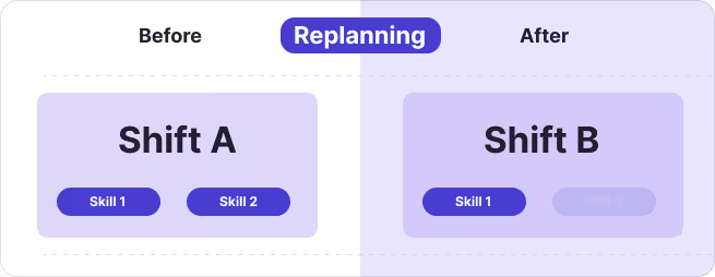
The shifts run at the same time. Ann has the skills for both. Should this count as disrupted?
- No, because from Ann's perspective the shifts start and end at the same time, and she's fully qualified to do either shift.
- Yes, because Ann's doing different work, because Skill 2 isn't needed in Shift B.
- Yes, because Shift A and Shift B are two different shifts and any reassignment is a disruption.
All three answers can be right, it just depends on your own operation or understanding of what "disruption" means.
More control over how you count disruptions
That's exactly why we recently added new configuration options to our disruption rules. You can now define whether shifts that overlap, or start/end within a set amount of time (e.g. 30 minutes) of each other should be counted as disrupted.
You can read more about that in our documentation.
If you have a specific use case in mind, reach out. We're always happy to extend the feature to fit your requirements.

Mixed Models in Timefold Solver: Combining Planning Variable Types in One Solution
Most planning problems fit neatly into one of two camps: you're either using @PlanningVariable to assign a single value to an entity, or @PlanningListVariable to build an ordered sequence. But real-world problems aren't always that tidy.
Sometimes a production line needs both an assigned operator and a queue of jobs to process. Sometimes you've got two different kinds of planning entities that each need their own variable type. And sometimes, the items inside a list are complex enough to need their own variables too. That's where mixed models come in.
A quick refresher on variable types
Before we get into mixed models, it helps to understand what we're mixing.
A basic planning variable holds a single value. Think assigning a Shift to an Employee, or a Room to a Meeting. It maps one entity to one value from a defined value range.
A list planning variable holds an ordered sequence of planning values. Think building a route for a Vehicle by assembling an ordered list of Visits. The solver decides both which values go in the list and in what order.
Mixed models let you use both in the same solution.
Pattern 1: Both variables on the same entity
The simplest form of a mixed model is a single planning entity that carries both a basic variable and a list variable.
@PlanningEntity
public class Line {

    @PlanningVariable
    private Operator operator;

    @PlanningListVariable
    private List<Job> jobs;
    // ...
}
Here, Line needs to know two things: which Operator is running it, and which Jobs it's processing (and in what order). Neither variable type alone could express this — you'd lose either the assignment or the sequence.
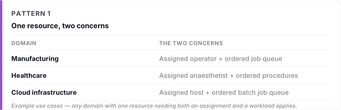
This pattern is useful any time a single resource needs both an assignment and a workload. A manufacturing floor is the obvious example: each production line is staffed by a single operator, but processes a variable list of jobs throughout the day. The operator assignment affects skill-based constraints (can this operator run this type of job?), while the job list drives throughput and scheduling constraints (do we have enough time? are dependencies respected?).
The same structure applies to a surgical theatre that needs an assigned anaesthetist and an ordered list of procedures for the day, or a cloud VM assigned to a physical host and running an ordered queue of batch jobs. One entity, two concerns, two variable types.
Pattern 2: Multiple entities, each with their own variable
The second pattern splits things across multiple planning entities. Each entity defines its own variable type independently.
@PlanningEntity
public class Line {

    @PlanningListVariable
    private List<Job> jobs;
    // ...
}

@PlanningEntity
public class LineOperation {

    @PlanningVariable
    private Operator operator;
    // ...
}
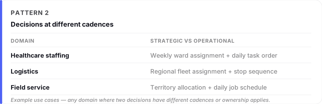
This works well when two decisions have genuinely different cadences or ownership: different lifecycles, different constraints, or different parts of the model that don't need to be tightly coupled on a single object.
Weekly staff rostering (assigning nurses to wards) combined with daily task scheduling (ordering tasks within a shift) is a natural fit. The roster changes weekly, the task list changes daily, and keeping them as separate entities means you can re-solve either without touching the other. Fleet assignment (which truck covers which region) paired with route planning (which stops that truck makes) follows the same logic: one decision is strategic, the other is operational, and conflating them in a single entity makes both harder to reason about.
Pattern 3: A child entity with its own variable
The third pattern goes one level deeper: the items inside a list variable are themselves planning entities, each carrying their own basic variable.
@PlanningEntity
public class Vehicle {

    @PlanningListVariable
    private List<Visit> visits;
    // ...
}

@PlanningEntity
public class Visit {

    @PlanningVariable
    private DropoffPoint dropOffBefore;
    // ...
}
Here, Vehicle owns an ordered list of Visits, that's your standard vehicle routing setup. But each Visit is also a @PlanningEntity in its own right, carrying a dropOffBefore variable that links it to a DropoffPoint.
This is what makes the Capacitated Vehicle Routing Problem with intermediate stops expressible. The parent shapes the route; the child refines each stop. That separation is what makes Pattern 3 so powerful, and what makes it the hardest to model without native support.
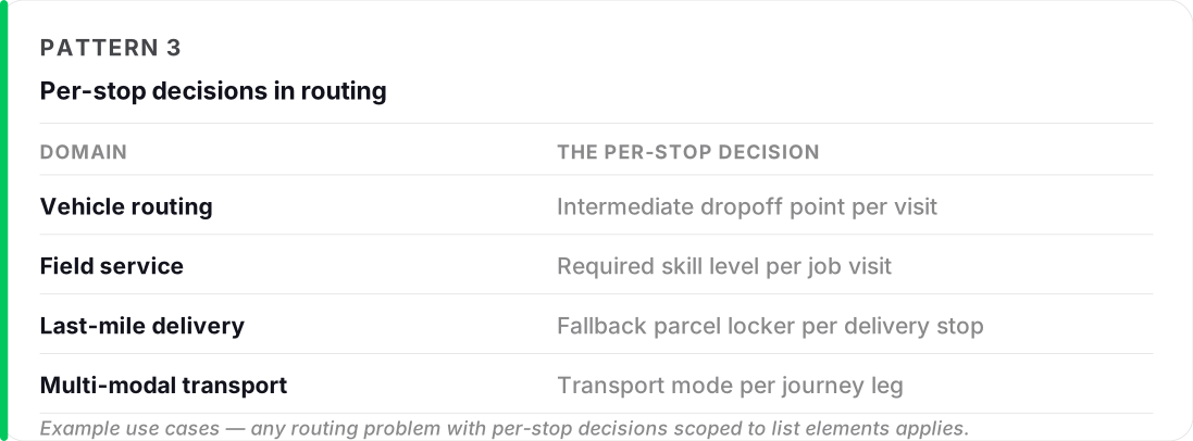
The common thread across use cases is decisions that are scoped to an element of a list rather than to the list as a whole. Consider last-mile delivery with parcel lockers: each Visit carries a @PlanningVariable for which locker to use as a fallback if no one is home. The route is solved at the vehicle level; the fallback assignment is solved at the visit level. Two decisions, two scopes, one clean model.
Multi-modal transport works the same way. An itinerary is a list of legs on a Traveller entity, but each leg independently decides its TransportMode (train, bus, or taxi) based on time, cost, and availability constraints. Without Pattern 3, you'd be encoding that per-leg decision somewhere it doesn't belong.
Wrapping up
Mixed models are one of those features that quietly unlocks a whole class of problems that used to require awkward workarounds. If you've been shoehorning your domain into a single variable type, it's worth asking whether your model is actually mixed and if so, just saying so explicitly.
Check out the Timefold Solver docs for the full reference on planning variables and mixed model configuration.

They're everywhere: Spotting optimization problems in the wild
I’ve been flying a bit more recently for speaking engagements. Dublin. CERN. A few other places in between. As fun as that sounds, it also means something else: A lot of time in airports.
Right now, as I’m writing this, I’m sitting at a gate waiting for my flight. My flight is delayed. The gate next to mine just changed. A crowd of people is collectively refreshing the airport app, hoping their boarding time magically moves forward so they don’t miss their connection.
I couldn’t help but smile and think: yep, this is a planning problem!
Over the past year, I’ve noticed something interesting about how I look at the world. I’ve written about it before, but the idea keeps coming back: Planning problems are everywhere.
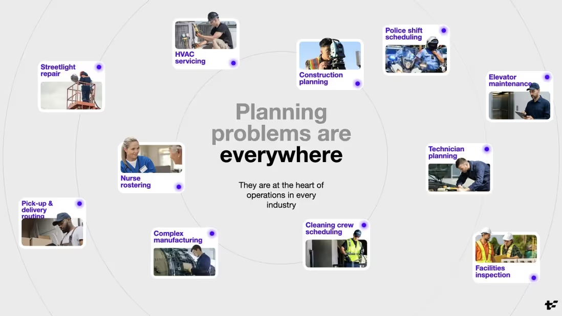
I’ve joked it is sort of a curse, once you start seeing them, you can’t really unsee them. And yet people underestimate just how common they are. When you start modelling these problems, you begin to notice something interesting: they all share the same structure.
Airports: A giant optimization puzzle
Airports might be one of the best examples.
When you think about everything that has to come together, it’s really a lot! Airports are actually running several optimization problems at the same time: gate assignment, crew scheduling, aircraft turnaround planning, runway slot allocation**,** and passenger connection protection. It’s almost a wonder airports work at all.

Yet people often remember just the negative and chaotic parts: the boarding delay, the last minute gate changes or the long lines at security.
Working with planning problems on a daily basis, I see things a little differently. Just understanding the immense complexity behind creating an initial plan already makes me feel calmer about the chaos.
Think about the decisions involved:
- Which gate should each flight use?
- Which crew can legally operate a flight after delays?
- How do we minimize missed connections?
- Where should incoming aircraft be parked?
- How do we re-route passengers when things go wrong?
Every delay or mishap ripples through that system of decisions, forcing the plan to be re-evaluated.
When the chaos hits, like it has around me writing this, I realize that this is just the result of a complex system constantly trying to adapt its plan as the situation changes.
And honestly, I can’t help but admire the attempt 🙂.
Irish breakfast, but optimized
Apparently I don’t even need to be fully awake to get bitten by the optimization bug.
After a busy evening speaking at a user group in Dublin and a shorter night than I hoped for, I dragged myself to a nearby breakfast restaurant to grab a proper Irish breakfast with a fellow optimization enthusiast.
As we were talking about the different projects we’d worked on, I became fascinated with the restaurant’s open kitchen layout. And once again, my mind drifted toward optimization.
A restaurant kitchen is basically a job scheduling system. Orders arrive dynamically. Each dish requires different preparation steps. The kitchen has limited resources: burners, ovens, chefs, and time.
The staff constantly make small scheduling decisions:
- Which order should be cooked first?
- Which dishes can run in parallel?
- How do we avoid one table waiting forever?
Experienced kitchens develop an intuition for it, but under the hood it resembles a classic job-shop scheduling problem.
And I couldn’t help but think how I’d model this problem as an optimization problem.
Sure, this kitchen is at a small scale. But structurally, it’s not that different from much larger systems.
CERN
I was lucky enough to be invited to speak at Voxxed Days CERN, which came with some awesome perks, including a guided tour through the facilities. You probably guessed it by now, but even here it made me wonder about the planning challenges behind the scenes.
- Scheduling maintenance for all different facilities
- Allocating compute resources for analysis jobs
- Coordinating experiments and detector usage

Even at one of the world’s most advanced research labs, the same fundamental problem appears again and again: “How do we allocate limited resources in the best possible way?”.
And of course, my brain was already buzzing with ways to optimize it.
Seeing the pattern
If you are involved with planning optimization solutions, a pattern starts to emerge that you can’t unsee. Many everyday systems share the same underlying structure:
- Resources (gates, buses, chefs, CPUs)
- Tasks (flights, routes, orders, jobs)
- Constraints (time limits, capacity, regulations)
- Objectives (speed, cost, fairness, efficiency)
…and the challenge becomes finding the best possible plan.
Optimization problems are just amazing puzzles… and quite addictive 🙂 The only downside is that once you start thinking this way, it becomes hard to stop.
You start seeing optimization problems everywhere:
In airports. In supermarkets. In conference schedules. In traffic lights. In restaurant kitchens.
Sometimes you’re just standing in line somewhere and suddenly catch yourself thinking:
This could be optimized!
Much to the dismay of my partner and friends, who occasionally see me drift off mid-conversation.
But when things go sideways, like delays at an airport, it also brings a strange kind of calm.
Because the chaos we see in the real world often isn’t chaos at all.
It’s a plan being repaired in real time.
And if you know how to look at it…
You start seeing optimization problems everywhere.

Solver 2.x: Java Platform Module System (JPMS) support.
We recently announced Timefold Solver 2.x, slated for somewhere later this month. It’s our first real major version since the fork (1.x was largely a package rename from the old OptaPlanner days) which means it’s finally time to address some issues we’ve been wanting to tackle for ages. One of them was modularity.
Java's public challenge
In Java, classes have a few visibility options. private, package-private, protected, and public. Large libraries often end up marking internal classes as public so different packages inside the library can interact. That’s exactly what happened in Timefold over the years.
As the codebase grew, some classes were technically public but never meant to be used by consumers. You’ve probably seen them:
ai.timefold.solver.core.*impl.*
Those packages contain implementation details of the solver. But since the classes were public, they were sometimes used anyway. From a user’s perspective, the reasoning is understandable: "If it’s public, why shouldn’t I use it?"
For years, Java lacked a visibility level that meant “public within this codebase, but not part of the supported API.” That changed with the introduction of Java Platform Module System (JPMS), which we will formally be supporting starting with Solver 2.0.
With JPMS we can explicitly choose which packages are exported and which remain internal.
module ai.timefold.solver.core {

    exports ai.timefold.solver.core.api.domain.common;
    exports ai.timefold.solver.core.api.domain.entity;
    exports ai.timefold.solver.core.api.domain.solution;
    exports ai.timefold.solver.core.api.domain.solution.cloner;

    // rest of file excluded
}
Exported packages are the supported API. Everything else stays internal. In other words:
public no longer means “public to the world.”
(If you run everything on the classpath instead of the modulepath, JPMS boundaries can still be bypassed. But for Solver 2.x, exported packages define the supported API.)
Why does this matter?
This change is mostly about clarity and long-term stability.
With explicit API boundaries we can:
- avoid accidental dependencies on internals
- refactor internal code more freely
- make upgrades less risky
Internal classes may change or disappear without notice. Exported packages are the stable API.
If you depend on internal classes
If your code imports packages containing .impl., you’re probably using internals.
Sometimes that happened because certain advanced use cases required it (e.g. Custom Moves). We’re actively working on replacing those patterns with supported public APIs.
If you have a legitimate use case that depends on internals, we’d like to hear about it. The goal isn’t to block anything, it’s to provide stable ways to do what you need without relying on implementation details.
If you’re using Timefold Solver and have concerns about internal classes you depend on, now is a great time to let us know.

How to prepare your data for scheduling optimization
Over the past decade, enterprises have invested heavily in understanding their data. Enterprises that have learned how to work with their data are in a strong position to forecast future needs, spot efficiencies, and act on opportunities.
If your field service organization has reached that point (or is getting close) there is one more door that structured, accessible data unlocks: optimization.
Not the vague, aspirational kind of optimization. The kind where you feed your technician availability, customer appointments, and job locations into an engine that produces the best schedule for the day - respecting every shift limit, skill requirement, time window, and lunch break - and returns it in seconds.
Optimization can be a key differentiator for many enterprises, but it is only as good as the data it consumes. In this post, we will walk through the data prerequisites for field service scheduling optimization, and explain why data readiness matters, which specific data you need (and where it typically lives), what opportunities open up once it is structured, and how to put it to work.
Why data readiness determines optimization success
A scheduling optimization engine is, at its core, a constraint solver. It takes a precise description of your planning problem (every technician, every job, every rule) and finds the best feasible assignment of work to people across time and space.
The operative word is precise. The engine cannot infer what it does not know. If a technician's lunch break is not in the data, the optimizer will schedule visits straight through it. If a customer's availability window is missing, the engine has no reason to avoid sending someone at 7 AM. If locations are inaccurate, travel time calculations fall apart, and the beautifully optimized route becomes fiction the moment a technician starts driving.
The quality of the output is bounded by the quality of the input. Organizations that have invested in structuring and owning their operational data are already past the hardest part. The remaining step is understanding which data optimization requires, and mapping it from where it already lives.
Which data do you need?
Field service optimization consumes three categories of data, each representing a different dimension of your operation. If you are familiar with spreadsheet-based scheduling, think of these as the tabs in your planning workbook. The difference? Instead of a planner manually cross-referencing them, an engine processes them all simultaneously.
1. Employee and vehicle data (the supply side)
This describes your workforce: who is available, when they work, what they can do, and when they need a break.
In the optimization model, each vehicle represents a technician and their transport for a given day. A vehicle record includes an id, the operating date, shift boundaries (minStartTime and maxEndTime), an optional maxSoftEndTime for overtime flexibility, the technician's skills, their startLocation and endLocation (typically home or a depot), a technicianRating, and any requiredBreaks for that day.
Breaks are defined within each vehicle's shift. Each break includes an id, a type (floating for a lunch that can slide within a window, or fixed for something like a medical appointment that cannot move), the date, a minStartTime and maxEndTime defining when the break can occur, and optionally a locationId if the technician needs to be somewhere specific for it.
Here is a simplified example of what this looks like as structured data:
{
 "id": "vehicle-1",
 "date": "2025-06-10",
 "minStartTime": "08:00",
 "maxEndTime": "17:00",
 "skills": ["HVAC", "electrical"],
 "startLocation": "loc-depot-01",
 "endLocation": "loc-depot-01",
 "requiredBreaks": [
   {
     "id": "break-1",
     "type": "floating",
     "minStartTime": "11:30",
     "maxEndTime": "13:30"
   }
 ]
}
This data typically lives across your HR or workforce management system (for shifts, skills, and PTO), your fleet management tool (for vehicle assignments), and sometimes a separate time-and-attendance platform. The key is being able to extract it per day, per technician, in a structured format.
2. Customer and work order data (the demand side)
This is every job that needs to happen: where, how long, when, and under what conditions.
Visits are the core unit of demand. Each visit includes an id, a name, a locationId linking it to a physical address, a serviceDuration (how long the job takes on-site), any requiredSkills the technician must have (matching the skills defined on the vehicle), a latestSlaEndTime if there is a contractual deadline, a priority level, and optionally a visitGroupId for jobs that require multiple technicians on-site simultaneously.
Each visit also includes one or more time windows defining when the customer is available. A time window has an id, a date, and a minStartTime and maxEndTime. A window of 10:00 to 13:00 means the technician must arrive within that range. Some visits may have multiple windows across different days, giving the optimizer flexibility in scheduling.
The completeness of your time windows and skill requirements often determines how much optimization headroom you actually have. If the engine does not know a customer is only available in the morning, it cannot avoid scheduling an afternoon arrival.
This data typically originates in your CRM, ERP, ticketing system, or field service management application.
3. Geographical data (the physical reality)
The third pillar ties everything together spatially. Without it, the optimizer has no concept of distance or travel time.
Locations are simple but critical: each record is an id, a latitude, and a longitude. These location IDs are referenced everywhere, in visits (where the job is), in vehicles (where the technician starts and ends their day), and in vehicle breaks (where a fixed appointment takes place).
This data lives in your CRM, address databases, or GIS systems. If you are still working primarily with street addresses, geocoding them into coordinate pairs is a prerequisite. Street-level addresses introduce ambiguity, a geocoded coordinate does not.
The optimization engine uses these coordinates to compute real-world travel times and distances between every relevant pair of points. The accuracy of your locations directly determines the accuracy of every route the engine produces.
What opportunities open up
Structuring and connecting these three data pillars is not just a checkbox exercise. It is the foundation for a fundamentally different way of operating.
From manual assembly to automated optimization. Today, dispatchers and planners spend hours each morning assembling routes by hand: Cross-referencing technician availability, customer windows, skill requirements, and geography, often in spreadsheets or on whiteboards. With structured data, this entire process becomes an API call. The engine considers every constraint simultaneously and returns an optimized plan in seconds.
From static plans to real-time replanning. A technician calls in sick at 8 AM. An emergency job arrives at 11:00. A visit runs an hour over. With structured, accessible data, you update the inputs and re-solve. The engine does not carry stale assumptions from the morning schedule. It takes the current reality and produces the best schedule from this point forward.
From gut feeling to explicit trade-offs. Should you minimize mileage or minimize overtime? Is SLA compliance more important than travel efficiency? With structured data and a configurable optimization model, these become tunable parameters with measurable impact. Not judgment calls made under pressure at 6 AM.
From siloed reporting to operational KPIs. Optimization outputs include metrics like total travel time, overtime incurred, visits completed versus unassigned, and utilization per technician. When your input data is clean and complete, these outputs become trustworthy enough to drive strategic decisions.
Putting it into practice
Most organizations will not find all three data pillars neatly organized in a single system. That is normal. The integration challenge is not about migrating everything into one database. It is about building a pipeline that assembles the optimization input from your existing sources and keeps it flowing.
Step 1: Map your sources. For each data entity (vehicles, vehicle breaks, visits, visit time windows, visit groups, locations), identify which system of record holds the authoritative version. Document where gaps exist: missing coordinates, incomplete time windows, skills not yet digitized.
Step 2: Close the gaps. Geocode addresses into coordinates. Ensure every technician's shift has explicit start and end times. Capture customer availability as structured time windows, not free-text notes. Define skills as a controlled vocabulary, not ad-hoc descriptions.
Step 3: Build the extraction layer. Create repeatable, automated exports from each source system. This could be API integrations, database queries, or scheduled file exports, whatever your systems support. The goal is to assemble a complete optimization dataset on demand, not through manual effort.
Step 4: Transform and submit. Map your extracted data into the structure the optimization engine expects (each vehicle with its shifts and breaks, each visit with its time windows and skills, each location as a coordinate pair) and POST it as a JSON payload to the API. Timefold's Field Service Routing API is stateless by design: it takes the full problem description, validates the input, solves it, and returns the optimized route plan. It does not store your data between runs. Each request is self-contained.
Step 5: Integrate the results. The response contains the optimized assignments - which visits land on which vehicle shift, in what order, with arrival times, departure times, and travel durations - plus KPIs summarizing overall plan quality. Push these assignments back into your dispatch system, mobile app, or field service management platform.
This stateless architecture is a deliberate choice that keeps you in control. Your data stays in your systems and you send only what is needed for each run. Any system that can make an HTTP request can integrate. When reality changes mid-day, you update the inputs and re-solve with no stale state. And every input and output is a complete, self-describing JSON document you can version, compare, and audit.
The takeaway
Data readiness is not a prerequisite you endure before the real work begins. For many organizations, it is the highest-leverage work and the foundation that makes forecasting, analysis, and optimization possible.
If your field service operation has been investing in structuring and owning its data, you are closer to optimization than you might think. The data you need already exists in your systems. The remaining step is connecting it.
And once it is connected, the results follow: less time on the road, more visits per day, fewer SLA breaches, and dispatchers freed to focus on exceptions rather than assembly. Not because of a magic algorithm, but because you gave the algorithm something precise to work with.
If you want to see how your data maps to the optimization model, explore Timefold's Field Service Routing documentation or start a trial on the platform.

Beyond self-scheduling: Balancing efficiency and autonomy in field service
Field service engineers don't resist technology because they fear change. They resist it because they've seen what happens when tools ignore how work actually gets done.
The objection we hear most often from operations leaders: "Our FSEs self-schedule. They won't accept a system that tells them where to go."
They're right to be cautious. But the choice isn't between autonomy and optimization. The best-performing field service organizations have found a third way.
The real problem with self-scheduling
Self-scheduling persists because it solves real problems. Engineers know their territories. They understand which customers need extra time. They've built relationships that smooth difficult service calls.
But self-scheduling also creates invisible costs:
- Route inefficiency compounds daily. An engineer who prefers to work east-to-west on Mondays might be adding 30 minutes of drive time without realizing it. Multiply that across a 50-person team and 250 working days.
- You have to trust blindly. The 80-20 rule applies here. Even if 80% of your employees schedule in good faith, there's always a minority that takes advantage of their freedom.
- The bigger picture stays invisible. Engineers often schedule only their immediate workload. They can't see that shifting Tuesday's route would unlock a more efficient Wednesday, or that a job they're avoiding this week will cascade into a scheduling nightmare next week. Longer planning horizons (across days, weeks, over the full team) reveal efficiencies that short-term, individual scheduling simply cannot surface.
- Skill mismatches go undetected. The best-qualified engineer for a complex repair might be in the next territory, but self-scheduling never surfaces that option.
- Preference conflicts accumulate. When three engineers all want Fridays off, or all avoid a difficult customer site, someone ends up overloaded, usually the newest team member who hasn't yet learned to game the system.
Can you afford the efficiency gap between what your team produces and what's mathematically possible?
Why FSEs push back on optimization
If optimization delivers clear efficiency gains, why the resistance?
Because most pure optimization tools treat engineers as interchangeable units to be deployed, not as skilled professionals with legitimate preferences and local knowledge.
When an algorithm assigns routes without explanation, engineers lose trust. When the schedule ignores a technician's need to pick up their child on Wednesdays, it fails the human test. When the system can't answer "why am I driving past this job to reach one further away?", it invites workarounds.
The result: engineers learn to game the system, dispatch overrides multiply, and the theoretical efficiency gains evaporate in practice.
This is a design failure, not an optimization failure.
The hybrid model: Optimal starting points, human control
The solution is not choosing between optimization and autonomy, but architecting systems that provide both.
Start with mathematically optimal schedules. The optimization engine generates routes that account for every constraint: geography, skills, time windows, equipment, SLAs, labor rules, and historical performance. This is objectively the best possible starting point, one that no human could calculate manually.
Present schedules as recommendations, not mandates. Engineers see their daily route with clear rationale. They can accept it as-is (which they probably should, since it's mathematically proven to be the most efficient solution given all constraints) or they can adjust it.
Enable controlled adjustments. If an engineer needs to be in a specific area on Wednesdays, they can set that preference. If they want to make a personal stop, they can adjust the route. If they see a better option based on local knowledge, they can make the change. Whether it's display as a drag-and-drop UI, or as re-optimize button with new constraints, engineers keep working on their terms.
Explainable AI: The trust architecture
Optimization without explanation is a black box. Engineers won't trust it, and operations leaders can't defend it.
For any scheduling decision, the system should articulate which constraints drove it: "You're assigned this job because you hold the required certification and are 12 minutes closer than the next qualified option." When trade-offs exist, show them: "Swapping these two stops would save 8 minutes of drive time but push the priority customer outside their SLA window."
When engineers can see why a schedule looks the way it does, resistance transforms into collaboration. Questions like "wouldn't it be better to go here first?" get answered in plain language, whether it's geographical clustering, skill-matching, time windows, or SLA requirements driving the sequence.
Engineers become partners in optimization rather than subjects of it.
Self-scheduling vs. optimized scheduling
Implementation without disruption
Even more than distrust, the strongest objection to any new system is disruption. Field service operations can't pause while IT rebuilds the scheduling stack. The right approach integrates optimization via API into existing dispatch systems and mobile apps. Why? Because engineers keep using familiar interfaces, and dispatchers keep their dashboards. Start with a pilot team, run optimization in parallel, compare results, and expand once the efficiency gains are proven.
A different conversation
The field service teams that succeed with optimization aren't the ones that override engineer autonomy. They're the ones that reframe the conversation.
Self-scheduling asks: "What route do I want to run today?"
Optimized scheduling asks: "Given everything we need to accomplish, what's the best version of the day I want to have?"
The second question is better. It respects engineer preferences while acknowledging that individual choices affect teammates, customers, and business outcomes.
When the optimization engine handles the combinatorial complexity, engineers can focus on what they do best: solving problems, building customer relationships, and applying the expertise that no algorithm can replicate.
That's the balance worth building toward.
[highlight]
Timefold provides scheduling optimization for field service operations through an API that integrates with existing dispatch systems. The platform produces explainable schedules with full constraint transparency, enabling teams to balance operational efficiency with workforce autonomy.
[highlight]

When scheduling works, everything works.
Less waste. More control. Teams that trust the plan.