Optimization algorithms
1. Introduction
1.1. Search space size in the real world
The number of possible solutions for a planning problem can be mind blowing. For example:
-
Four queens has
256possible solutions (4^4) and two optimal solutions. -
Five queens has
3125possible solutions (5^5) and one optimal solution. -
Eight queens has
16777216possible solutions (8^8) and 92 optimal solutions. -
64 queens has more than
10^115possible solutions (64^64). -
Most real-life planning problems have an incredible number of possible solutions and only one or a few optimal solutions.
For comparison: the minimal number of atoms in the known universe (10^80). As a planning problem gets bigger, the search space tends to blow up really fast. Adding only one extra planning entity or planning value can heavily multiply the running time of some algorithms. Calculating the number of possible solutions depends on the design of the domain model:

|
This search space size calculation includes infeasible solutions (if they can be represented by the model), because:
Even in cases where adding some of the hard constraints in the formula is practical, the resulting search space is still huge. |
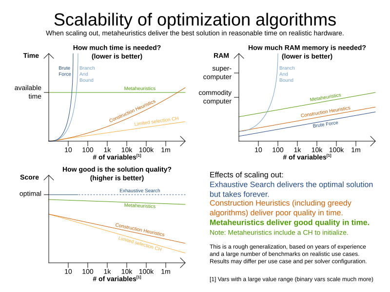
An algorithm that checks every possible solution (even with pruning, such as in Branch And Bound) can easily run for billions of years on a single real-life planning problem. The aim is to find the best solution in the available timeframe. Planning competitions (such as the International Timetabling Competition) show that Local Search variations (Tabu Search, Simulated Annealing, Late Acceptance, …) usually perform best for real-world problems given real-world time limitations.
1.2. Does Timefold Solver find the optimal solution?
The business wants the optimal solution, but they also have other requirements:
-
Scale out: Large production data sets must not crash and have also good results.
-
Optimize the right problem: The constraints must match the actual business needs.
-
Available time: The solution must be found in time, before it becomes useless to execute.
-
Reliability: Every data set must have at least a decent result (better than a human planner).
Given these requirements, and despite the promises of some salesmen, it is usually impossible for anyone or anything to find the optimal solution. Therefore, Timefold Solver focuses on finding the best solution in available time.
The nature of NP-complete problems make scaling a prime concern.
|
The quality of a result from a small data set is no indication of the quality of a result from a large data set. |
Scaling issues cannot be mitigated by hardware purchases later on. Start testing with a production sized data set as soon as possible. Do not assess quality on small data sets (unless production encounters only such data sets). Instead, solve a production sized data set and compare the results of longer executions, different algorithms and - if available - the human planner.
1.3. Supported optimization algorithms
Timefold Solver supports three families of optimization algorithms: Exhaustive Search, Construction Heuristics and Metaheuristics. In practice, Metaheuristics (in combination with Construction Heuristics to initialize) are the recommended choice:
Each of these algorithm families have multiple optimization algorithms:
| Algorithm | Scalable? | Optimal? | Easy to use? | Tweakable? | Requires CH? |
|---|---|---|---|---|---|
Exhaustive Search (ES) |
|||||
0/5 |
5/5 |
5/5 |
0/5 |
No |
|
0/5 |
5/5 |
4/5 |
2/5 |
No |
|
Construction heuristics (CH) |
|||||
5/5 |
1/5 |
5/5 |
1/5 |
No |
|
5/5 |
2/5 |
4/5 |
2/5 |
No |
|
5/5 |
2/5 |
4/5 |
2/5 |
No |
|
5/5 |
2/5 |
4/5 |
2/5 |
No |
|
5/5 |
2/5 |
4/5 |
2/5 |
No |
|
5/5 |
2/5 |
4/5 |
2/5 |
No |
|
3/5 |
2/5 |
5/5 |
2/5 |
No |
|
3/5 |
2/5 |
5/5 |
2/5 |
No |
|
Metaheuristics (MH) |
|||||
Local Search (LS) |
|||||
5/5 |
2/5 |
4/5 |
3/5 |
Yes |
|
5/5 |
4/5 |
3/5 |
5/5 |
Yes |
|
5/5 |
4/5 |
2/5 |
5/5 |
Yes |
|
5/5 |
4/5 |
3/5 |
5/5 |
Yes |
|
5/5 |
4/5 |
3/5 |
5/5 |
Yes |
|
5/5 |
4/5 |
3/5 |
5/5 |
Yes |
|
3/5 |
3/5 |
2/5 |
5/5 |
Yes |
|
To learn more about metaheuristics, see Essentials of Metaheuristics or Clever Algorithms.
1.4. Which optimization algorithms should I use?
The best optimization algorithms configuration to use depends heavily on your use case. However, this basic procedure provides a good starting configuration that will produce better than average results.
-
Start with a quick configuration that involves little or no configuration and optimization code: See First Fit.
-
Next, implement planning entity difficulty comparison and turn it into First Fit Decreasing.
-
Next, add Late Acceptance behind it:
-
First Fit Decreasing.
-
At this point, the return on invested time lowers and the result is likely to be sufficient.
However, this can be improved at a lower return on invested time. Use the Benchmarker and try a couple of different Tabu Search, Simulated Annealing and Late Acceptance configurations, for example:
-
First Fit Decreasing: Tabu Search.
Use the Benchmarker to improve the values for the size parameters.
Other experiments can also be run. For example, the following multiple algorithms can be combined together:
-
First Fit Decreasing
-
Late Acceptance (relatively long time)
-
Tabu Search (relatively short time)
2. Architecture overview
Timefold Solver combines optimization algorithms (metaheuristics, …) with score calculation by a score calculation engine. This combination is very efficient, because:
-
A score calculation engine, is great for calculating the score of a solution of a planning problem. It makes it easy and scalable to add additional soft or hard constraints. It does incremental score calculation (deltas) without any extra code. However it tends to be not suitable to actually find new solutions.
-
An optimization algorithm is great at finding new improving solutions for a planning problem, without necessarily brute-forcing every possibility. However, it needs to know the score of a solution and offers no support in calculating that score efficiently.

2.1. Power tweaking or default parameter values
Many optimization algorithms have parameters that affect results and scalability. Timefold Solver applies configuration by exception, so all optimization algorithms have default parameter values. This is very similar to the Garbage Collection parameters in a JVM: most users have no need to tweak them, but power users often do.
The default parameter values are sufficient for many cases (and especially for prototypes), but if development time allows, it may be beneficial to power tweak them with the benchmarker for better results and scalability on a specific use case. The documentation for each optimization algorithm also declares the advanced configuration for power tweaking.
|
The default value of parameters will change between minor versions, to improve them for most users. The advanced configuration can be used to prevent unwanted changes, however, this is not recommended. |
2.2. Solver phase
A Solver can use multiple optimization algorithms in sequence.
Each optimization algorithm is represented by one solver Phase.
There is never more than one Phase solving at the same time.
|
Some |
Here is a configuration that runs three phases in sequence:
<solver xmlns="https://timefold.ai/xsd/solver" xmlns:xsi="http://www.w3.org/2001/XMLSchema-instance"
    xsi:schemaLocation="https://timefold.ai/xsd/solver https://timefold.ai/xsd/solver/solver.xsd">
  ...
  <constructionHeuristic>
    ... <!-- First phase: First Fit Decreasing -->
  </constructionHeuristic>
  <localSearch>
    ... <!-- Second phase: Late Acceptance -->
  </localSearch>
  <localSearch>
    ... <!-- Third phase: Tabu Search -->
  </localSearch>
</solver>
The solver phases are run in the order defined by solver configuration.
-
When the first
Phaseterminates, the secondPhasestarts, and so on. -
When the last
Phaseterminates, theSolverterminates.
Usually, a Solver will first run a construction heuristic and then run one or multiple metaheuristics:
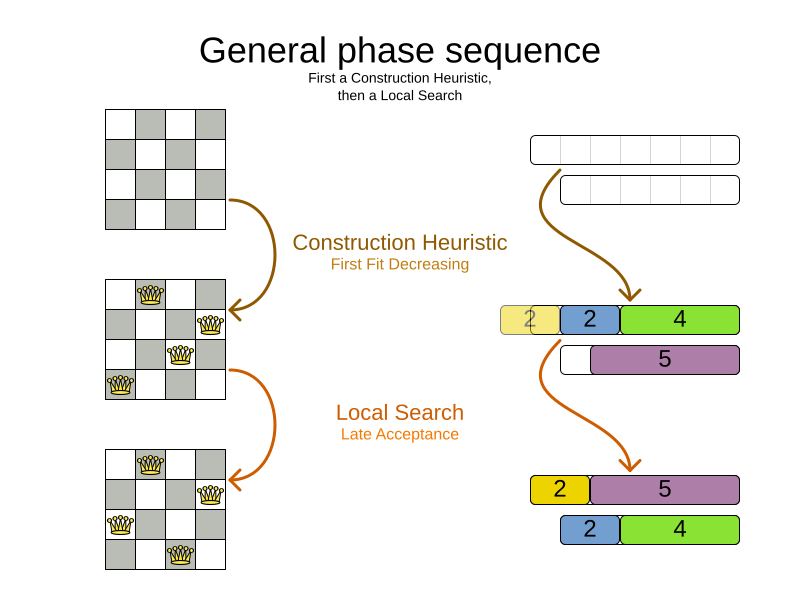
If no phases are configured, Timefold Solver will default to a Construction Heuristic phase followed by a Local Search phase.
Some phases (especially construction heuristics) will terminate automatically.
Other phases (especially metaheuristics) will only terminate if the Phase is configured to terminate:
<solver xmlns="https://timefold.ai/xsd/solver" xmlns:xsi="http://www.w3.org/2001/XMLSchema-instance"
    xsi:schemaLocation="https://timefold.ai/xsd/solver https://timefold.ai/xsd/solver/solver.xsd">
  ...
  <termination><!-- Solver termination -->
    <secondsSpentLimit>90</secondsSpentLimit>
  </termination>
  <localSearch>
    <termination><!-- Phase termination -->
      <secondsSpentLimit>60</secondsSpentLimit><!-- Give the next phase a chance to run too, before the Solver terminates -->
    </termination>
    ...
  </localSearch>
  <localSearch>
    ...
  </localSearch>
</solver>
If the Solver terminates (before the last Phase terminates itself),
the current phase is terminated and all subsequent phases will not run.
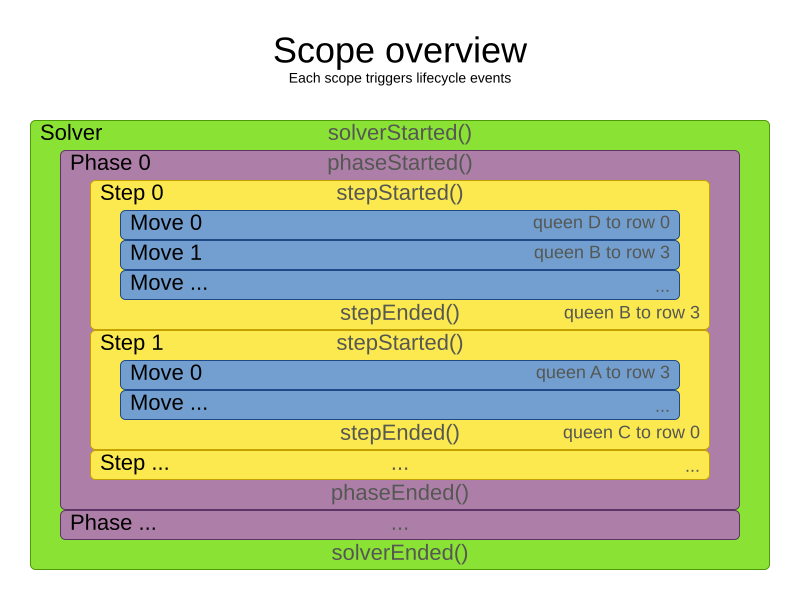
2.3. Scope overview
A solver will iteratively run phases. Each phase will usually iteratively run steps. Each step, in turn, usually iteratively runs moves. These form four nested scopes:
-
Solver
-
Phase
-
Step
-
Move
Configure logging to display the log messages of each scope.
2.4. Termination
Not all phases terminate automatically and may take a significant amount of time.
A Solver can be terminated synchronously by up-front configuration, or asynchronously from another thread.
Metaheuristic phases in particular need to be instructed to stop solving. This can be because of a number of reasons, for example, if the time is up, or the perfect score has been reached just before its solution is used. Finding the optimal solution cannot be relied on (unless you know the optimal score), because a metaheuristic algorithm is generally unaware of the optimal solution.
This is not an issue for real-life problems, as finding the optimal solution may take more time than is available. Finding the best solution in the available time is the most important outcome.
|
If no termination is configured (and a metaheuristic algorithm is used), the |
For synchronous termination, configure a Termination on a Solver or a Phase when it needs to stop.
Every Termination can calculate a time gradient (needed for some optimization algorithms),
which is a ratio between the time already spent solving and the estimated entire solving time of the Solver or Phase.
2.4.1. Time spent termination
Terminates when an amount of time has been used.
  <termination>
    <!-- 2 minutes and 30 seconds in ISO 8601 format P[n]Y[n]M[n]DT[n]H[n]M[n]S -->
    <spentLimit>PT2M30S</spentLimit>
  </termination>
Alternatively to a java.util.Duration in ISO 8601 format, you can also use:
-
Milliseconds
<termination> <millisecondsSpentLimit>500</millisecondsSpentLimit> </termination> -
Seconds
<termination> <secondsSpentLimit>10</secondsSpentLimit> </termination> -
Minutes
<termination> <minutesSpentLimit>5</minutesSpentLimit> </termination> -
Hours
<termination> <hoursSpentLimit>1</hoursSpentLimit> </termination> -
Days
  <termination>
    <daysSpentLimit>2</daysSpentLimit>
  </termination>
Multiple time types can be used together, for example to configure 150 minutes, either configure it directly:
  <termination>
    <minutesSpentLimit>150</minutesSpentLimit>
  </termination>
Or use a combination that sums up to 150 minutes:
  <termination>
    <hoursSpentLimit>2</hoursSpentLimit>
    <minutesSpentLimit>30</minutesSpentLimit>
</termination>|
This
|
2.4.2. Unimproved time spent termination
Terminates when the best score has not improved in a specified amount of time. Each time a new best solution is found, the timer basically resets.
  <localSearch>
    <termination>
      <!-- 2 minutes and 30 seconds in ISO 8601 format P[n]Y[n]M[n]DT[n]H[n]M[n]S -->
      <unimprovedSpentLimit>PT2M30S</unimprovedSpentLimit>
    </termination>
  </localSearch>
Alternatively to a java.util.Duration in ISO 8601 format, you can also use:
-
Milliseconds
<localSearch> <termination> <unimprovedMillisecondsSpentLimit>500</unimprovedMillisecondsSpentLimit> </termination> </localSearch> -
Seconds
<localSearch> <termination> <unimprovedSecondsSpentLimit>10</unimprovedSecondsSpentLimit> </termination> </localSearch> -
Minutes
<localSearch> <termination> <unimprovedMinutesSpentLimit>5</unimprovedMinutesSpentLimit> </termination> </localSearch> -
Hours
<localSearch> <termination> <unimprovedHoursSpentLimit>1</unimprovedHoursSpentLimit> </termination> </localSearch> -
Days
  <localSearch>
    <termination>
      <unimprovedDaysSpentLimit>1</unimprovedDaysSpentLimit>
    </termination>
  </localSearch>
Just like time spent termination, combinations are summed up.
It is preffered to configure this termination on a specific Phase (such as <localSearch>) instead of on the Solver itself.
Several phases, such as construction heuristics, do not count towards this termination because they only trigger new best solution events when they are done. If such a phase is encountered, the termination is disabled and when the next phase is started, the termination is enabled again and the timer resets back to zero. In the most typical case, where a local search phase follows a construction heuristic phase, the termination will only trigger if the local search phase does not improve the best solution for the specified time.
|
This
|
Optionally, configure a score difference threshold by which the best score must improve in the specified time.
For example, if the score doesn’t improve by at least 100 soft points every 30 seconds or less, it terminates:
  <localSearch>
    <termination>
      <unimprovedSecondsSpentLimit>30</unimprovedSecondsSpentLimit>
      <unimprovedScoreDifferenceThreshold>0hard/100soft</unimprovedScoreDifferenceThreshold>
    </termination>
  </localSearch>
If the score improves by 1 hard point and drops 900 soft points, it’s still meets the threshold,
because 1hard/-900soft is larger than the threshold 0hard/100soft.
On the other hand, a threshold of 1hard/0soft is not met by any new best solution
that improves 1 hard point at the expense of 1 or more soft points,
because 1hard/-100soft is smaller than the threshold 1hard/0soft.
To require a feasibility improvement every 30 seconds while avoiding the pitfall above,
use a wildcard * for lower score levels that are allowed to deteriorate if a higher score level improves:
  <localSearch>
    <termination>
      <unimprovedSecondsSpentLimit>30</unimprovedSecondsSpentLimit>
      <unimprovedScoreDifferenceThreshold>1hard/*soft</unimprovedScoreDifferenceThreshold>
    </termination>
  </localSearch>
This effectively implies a threshold of 1hard/-2147483648soft, because it relies on Integer.MIN_VALUE.
2.4.3. BestScoreTermination
BestScoreTermination terminates when a certain score has been reached.
Use this Termination where the perfect score is known,
for example for four queens (which uses a SimpleScore):
  <termination>
    <bestScoreLimit>0</bestScoreLimit>
  </termination>
A planning problem with a HardSoftScore may look like this:
  <termination>
    <bestScoreLimit>0hard/-5000soft</bestScoreLimit>
  </termination>
A planning problem with a BendableScore with three hard levels and one soft level may look like this:
  <termination>
    <bestScoreLimit>[0/0/0]hard/[-5000]soft</bestScoreLimit>
  </termination>
In this instance, Termination once a feasible solution has been reached is not practical because it requires a bestScoreLimit such as 0hard/-2147483648soft. Use the next termination instead.
2.4.4. BestScoreFeasibleTermination
Terminates as soon as a feasible solution has been discovered.
  <termination>
    <bestScoreFeasible>true</bestScoreFeasible>
  </termination>
This Termination is usually combined with other terminations.
2.4.5. StepCountTermination
Terminates when a number of steps has been reached. This is useful for hardware performance independent runs.
  <localSearch>
    <termination>
      <stepCountLimit>100</stepCountLimit>
    </termination>
  </localSearch>
This Termination can only be used for a Phase (such as <localSearch>), not for the Solver itself.
2.4.6. UnimprovedStepCountTermination
Terminates when the best score has not improved in a number of steps. This is useful for hardware performance independent runs.
  <localSearch>
    <termination>
      <unimprovedStepCountLimit>100</unimprovedStepCountLimit>
    </termination>
  </localSearch>
If the score has not improved recently, it is unlikely to improve in a reasonable timeframe. It has been observed that once a new best solution is found (even after a long time without improvement on the best solution), the next few steps tend to improve the best solution.
This Termination can only be used for a Phase (such as <localSearch>), not for the Solver itself.
2.4.7. ScoreCalculationCountTermination
ScoreCalculationCountTermination terminates when a number of score calculations have been reached.
This is often the sum of the number of moves and the number of steps.
This is useful for benchmarking.
  <termination>
    <scoreCalculationCountLimit>100000</scoreCalculationCountLimit>
  </termination>
Switching EnvironmentMode can heavily impact when this termination ends.
2.4.8. Combining multiple terminations
Terminations can be combined, for example: terminate after 100 steps or if a score of 0 has been reached:
  <termination>
    <terminationCompositionStyle>OR</terminationCompositionStyle>
    <bestScoreLimit>0</bestScoreLimit>
    <stepCountLimit>100</stepCountLimit>
  </termination>
Alternatively you can use AND, for example: terminate after reaching a feasible score of at least -100 and no improvements in 5 steps:
  <termination>
    <terminationCompositionStyle>AND</terminationCompositionStyle>
    <bestScoreLimit>-100</bestScoreLimit>
    <unimprovedStepCountLimit>5</unimprovedStepCountLimit>
  </termination>
This example ensures it does not just terminate after finding a feasible solution, but also completes any obvious improvements on that solution before terminating.
2.4.9. Asynchronous termination from another thread
Asynchronous termination cannot be configured by a Termination as it is impossible to predict when and if it will occur.
For example, a user action or a server restart could require a solver to terminate earlier than predicted.
To terminate a solver from another thread asynchronously
call the terminateEarly() method from another thread:
solver.terminateEarly();The solver then terminates at its earliest convenience.
After termination, the Solver.solve(Solution) method returns in the solver thread (which is the original thread that called it).
|
When an To guarantee a graceful shutdown of a thread pool that contains solver threads,
an interrupt of a solver thread has the same effect as calling |
2.5. SolverEventListener
Each time a new best solution is found, a new BestSolutionChangedEvent is fired in the Solver thread.
To listen to such events, add a SolverEventListener to the Solver:
public interface Solver<Solution_> {
    ...

    void addEventListener(SolverEventListener<S> eventListener);
    void removeEventListener(SolverEventListener<S> eventListener);

}
The BestSolutionChangedEvent's newBestSolution may not be initialized or feasible.
Use the isFeasible() method on BestSolutionChangedEvent's new best Score to detect such cases.
Use Score.isSolutionInitialized() instead of Score.isFeasible() to only ignore uninitialized solutions,
but also accept infeasible solutions.
|
The |
2.6. Custom solver phase
Run a custom optimization algorithm between phases or before the first phase to initialize the solution, or to get a better score quickly.
You will still want to reuse the score calculation.
For example, to implement a custom Construction Heuristic without implementing an entire Phase.
|
Most of the time, a custom solver phase is not worth the development time investment.
Constructions Heuristics are configurable,
|
The CustomPhaseCommand interface appears as follows:
public interface CustomPhaseCommand<Solution_> {
    ...

    void changeWorkingSolution(ScoreDirector<Solution_> scoreDirector);

}|
Any change on the planning entities in a |
|
Do not change any of the problem facts in a |
Configure the CustomPhaseCommand in the solver configuration:
<solver xmlns="https://timefold.ai/xsd/solver" xmlns:xsi="http://www.w3.org/2001/XMLSchema-instance"
    xsi:schemaLocation="https://timefold.ai/xsd/solver https://timefold.ai/xsd/solver/solver.xsd">
  ...
  <customPhase>
    <customPhaseCommandClass>...MyCustomPhase</customPhaseCommandClass>
  </customPhase>
  ... <!-- Other phases -->
</solver>
Configure multiple customPhaseCommandClass instances to run them in sequence.
|
If the changes of a |
|
If the |
To configure values of a CustomPhaseCommand dynamically in the solver configuration
(so the Benchmarker can tweak those parameters),
add the customProperties element and use custom properties:
  <customPhase>
    <customPhaseCommandClass>...MyCustomPhase</customPhaseCommandClass>
    <customProperties>
      <property name="mySelectionSize" value="5"/>
    </customProperties>
  </customPhase>
2.7. No change solver phase
In rare cases, it’s useful not to run any solver phases.
But by default, configuring no phase will trigger running the default phases.
To avoid those, configure a NoChangePhase:
<solver xmlns="https://timefold.ai/xsd/solver" xmlns:xsi="http://www.w3.org/2001/XMLSchema-instance"
    xsi:schemaLocation="https://timefold.ai/xsd/solver https://timefold.ai/xsd/solver/solver.xsd">
  ...
  <noChangePhase/>
</solver>
3. Move and neighborhood selection
3.1. Move and neighborhood introduction
3.1.1. What is a Move?
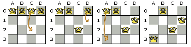
A Move is a change (or set of changes) from a solution A to a solution B.
For example, the move below changes queen C from row 0 to row 2:
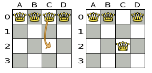
The new solution is called a neighbor of the original solution, because it can be reached in a single Move.
Although a single move can change multiple queens,
the neighbors of a solution should always be a tiny subset of all possible solutions.
For example, on that original solution, these are all possible changeMoves:
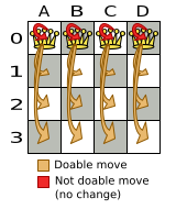
If we ignore the four changeMoves that have no impact and are therefore not doable, we can see that the number of moves is n * (n - 1) = 12.
This is far less than the number of possible solutions, which is n ^ n = 256.
As the problem scales out, the number of possible moves increases far less than the number of possible solutions.
Yet, in four changeMoves or less we can reach any solution.
For example we can reach a very different solution in three changeMoves:
|
There are many other types of moves besides A |
All optimization algorithms use Moves to transition from one solution to a neighbor solution.
Therefore, all the optimization algorithms are confronted with Move selection: the craft of creating and iterating moves efficiently and the art of finding the most promising subset of random moves to evaluate first.
3.1.2. What is a MoveSelector?
A MoveSelector's main function is to create Iterator<Move> when needed.
An optimization algorithm will iterate through a subset of those moves.
Here’s an example how to configure a changeMoveSelector for the optimization algorithm Local Search:
  <localSearch>
    <changeMoveSelector/>
    ...
  </localSearch>
Out of the box, this works and all properties of the changeMoveSelector are defaulted sensibly (unless that fails fast due to ambiguity). On the other hand, the configuration can be customized significantly for specific use cases.
For example: you might want to configure a filter to discard pointless moves.
3.1.3. Subselecting of entities, values, and other moves
To create a Move, a MoveSelector needs to select one or more planning entities and/or planning values to move.
Just like MoveSelectors, EntitySelectors and ValueSelectors need to support a similar feature set (such as scalable just-in-time selection). Therefore, they all implement a common interface Selector and they are configured similarly.
A MoveSelector is often composed out of EntitySelectors, ValueSelectors or even other MoveSelectors, which can be configured individually if desired:
    <unionMoveSelector>
      <changeMoveSelector>
        <entitySelector>
          ...
        </entitySelector>
        <valueSelector>
          ...
        </valueSelector>
        ...
      </changeMoveSelector>
      <swapMoveSelector>
        ...
      </swapMoveSelector>
    </unionMoveSelector>
Together, this structure forms a Selector tree:

The root of this tree is a MoveSelector which is injected into the optimization algorithm implementation to be (partially) iterated in every step.
3.2. Generic MoveSelectors
3.2.1. Generic MoveSelectors overview
| Name | Description | toString() example |
|---|---|---|
Change 1 entity’s variable |
|
|
Swap all variables of 2 entities |
|
|
Change a set of entities with the same value |
|
|
Swap 2 sets of entities with the same values |
|
|
Move a list element to a different index or to another entity’s list variable |
|
|
Swap 2 list elements |
|
|
Move a subList from one position to another |
|
|
Swap 2 subLists |
|
|
Select an entity, remove k edges from its list variable, add k new edges from the removed endpoints |
|
|
Swap 2 tails chains |
|
|
Cut a subchain and paste it into another chain |
|
|
Swap 2 subchains |
|
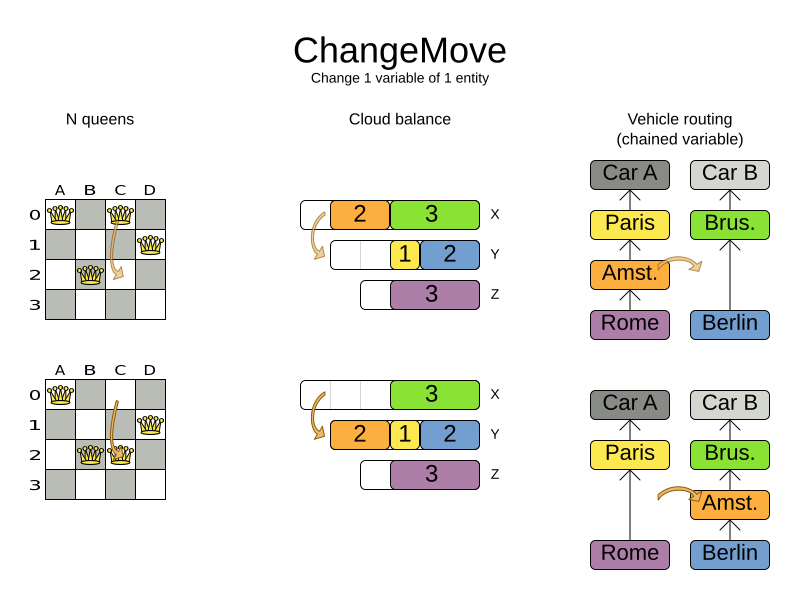
3.2.2. ChangeMoveSelector
For one planning variable, the ChangeMove selects one planning entity and one planning value and assigns the entity’s variable to that value.
Simplest configuration:
<changeMoveSelector/>If there are multiple entity classes or multiple planning variables for one entity class, a simple configuration will automatically unfold into a union of ChangeMove selectors for every planning variable.
Advanced configuration:
    <changeMoveSelector>
      ... <!-- Normal selector properties -->
      <entitySelector>
        <entityClass>...Lecture</entityClass>
        ...
      </entitySelector>
      <valueSelector variableName="room">
        ...
      </valueSelector>
    </changeMoveSelector>
A ChangeMove is the finest grained move.
|
Almost every |
This move selector only supports phase or solver caching if it doesn’t apply on a chained variable.
3.2.3. SwapMoveSelector
The SwapMove selects two different planning entities and swaps the planning values of all their planning variables.

Although a SwapMove on a single variable is essentially just two ChangeMoves,
it’s often the winning step in cases that the first of the two ChangeMoves would not win
because it leaves the solution in a state with broken hard constraints.
For example: swapping the room of two lectures doesn’t bring the solution in an intermediate state where both lectures are in the same room which breaks a hard constraint.
Simplest configuration:
<swapMoveSelector/>If there are multiple entity classes, a simple configuration will automatically unfold into a union of SwapMove selectors for every entity class.
Advanced configuration:
    <swapMoveSelector>
      ... <!-- Normal selector properties -->
      <entitySelector>
        <entityClass>...Lecture</entityClass>
        ...
      </entitySelector>
      <secondaryEntitySelector>
        <entityClass>...Lecture</entityClass>
        ...
      </secondaryEntitySelector>
      <variableNameIncludes>
        <variableNameInclude>room</variableNameInclude>
        <variableNameInclude>...</variableNameInclude>
      </variableNameIncludes>
    </swapMoveSelector>
The secondaryEntitySelector is rarely needed: if it is not specified, entities from the same entitySelector are swapped.
If one or more variableNameInclude properties are specified, not all planning variables will be swapped, but only those specified.
This move selector only supports phase or solver caching if it doesn’t apply on any chained variables.
3.2.4. Pillar-based move selectors
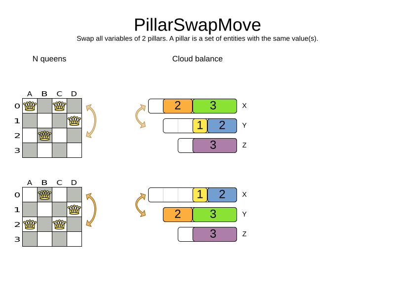
A pillar is a set of planning entities which have the same planning value(s) for their planning variable(s).
PillarChangeMoveSelector
The PillarChangeMove selects one entity pillar (or subset of those) and changes the value of one variable (which is the same for all entities) to another value.

In the example above, queen A and C have the same value (row 0) and are moved to row 2. Also the yellow and blue process have the same value (computer Y) and are moved to computer X.
Simplest configuration:
<pillarChangeMoveSelector/>Advanced configuration:
    <pillarChangeMoveSelector>
      <subPillarType>SEQUENCE</subPillarType>
      <subPillarSequenceComparatorClass>...ShiftComparator</subPillarSequenceComparatorClass>
      ... <!-- Normal selector properties -->
      <pillarSelector>
        <entitySelector>
          <entityClass>...Shift</entityClass>
          ...
        </entitySelector>
        <minimumSubPillarSize>1</minimumSubPillarSize>
        <maximumSubPillarSize>1000</maximumSubPillarSize>
      </pillarSelector>
      <valueSelector variableName="employee">
        ...
      </valueSelector>
    </pillarChangeMoveSelector>
For a description of subPillarType and related properties, please refer to Subpillars.
The other properties are explained in changeMoveSelector. This move selector does not support phase or solver caching and step caching scales badly memory wise.
PillarSwapMoveSelector
The PillarSwapMove selects two different entity pillars and swaps the values of all their variables for all their entities.
Simplest configuration:
<pillarSwapMoveSelector/>Advanced configuration:
    <pillarSwapMoveSelector>
      <subPillarType>SEQUENCE</subPillarType>
      <subPillarSequenceComparatorClass>...ShiftComparator</subPillarSequenceComparatorClass>
      ... <!-- Normal selector properties -->
      <pillarSelector>
        <entitySelector>
          <entityClass>...Shift</entityClass>
          ...
        </entitySelector>
        <minimumSubPillarSize>1</minimumSubPillarSize>
        <maximumSubPillarSize>1000</maximumSubPillarSize>
      </pillarSelector>
      <secondaryPillarSelector>
        <entitySelector>
          ...
        </entitySelector>
        ...
      </secondaryPillarSelector>
      <variableNameIncludes>
        <variableNameInclude>employee</variableNameInclude>
        <variableNameInclude>...</variableNameInclude>
      </variableNameIncludes>
    </pillarSwapMoveSelector>
For a description of subPillarType and related properties, please refer to sub pillars.
The secondaryPillarSelector is rarely needed: if it is not specified, entities from the same pillarSelector are swapped.
The other properties are explained in swapMoveSelector and pillarChangeMoveSelector. This move selector does not support phase or solver caching and step caching scales badly memory wise.
Sub pillars
A sub pillar is a subset of entities that share the same value(s) for their variable(s).
For example if queen A, B, C and D are all located on row 0, they are a pillar and [A, D] is one of the many sub pillars.
There are several ways how sub pillars can be selected by the subPillarType property:
-
ALL(default) selects all possible sub pillars. -
SEQUENCElimits selection of sub pillars to Sequential sub pillars. -
NONEnever selects any sub pillars.
If sub pillars are enabled, the pillar itself is also included and the properties minimumSubPillarSize (defaults to 1) and maximumSubPillarSize (defaults to infinity) limit the size of the selected (sub) pillar.
|
The number of sub pillars of a pillar is exponential to the size of the pillar.
For example a pillar of size 32 has |
Sequential sub pillars
Sub pillars can be sorted with a Comparator. A sequential sub pillar is a continuous subset of its sorted base pillar.
For example, if an employee has shifts on Monday (M), Tuesday (T), and Wednesday (W),
they are a pillar and only the following are its sequential sub pillars: [M], [T], [W], [M, T], [T, W], [M, T, W].
But [M, W] is not a sub pillar in this case, as there is a gap on Tuesday.
Sequential sub pillars apply to both Pillar change move and Pillar swap move. A minimal configuration looks like this:
    <pillar...MoveSelector>
      <subPillarType>SEQUENCE</subPillarType>
    </pillar...MoveSelector>
In this case, the entity being operated on must implement the Comparable interface. The size of sub pillars will not be limited in any way.
An advanced configuration looks like this:
    <pillar...MoveSelector>
      ...
      <subPillarType>SEQUENCE</subPillarType>
      <subPillarSequenceComparatorClass>...ShiftComparator</subPillarSequenceComparatorClass>
      <pillarSelector>
        ...
        <minimumSubPillarSize>1</minimumSubPillarSize>
        <maximumSubPillarSize>1000</maximumSubPillarSize>
      </pillarSelector>
      ...
    </pillar...MoveSelector>
In this case, the entity being operated on need not be Comparable.
The given subPillarSequenceComparatorClass is used to establish the sequence instead.
Also, the size of the sub pillars is limited in length of up to 1000 entities.
3.2.5. Move selectors for list variables
ListChangeMoveSelector
The ListChangeMoveSelector selects an element from a list variable’s value range and moves it from its current position to a new one.
Simplest configuration:
<listChangeMoveSelector/>Advanced configuration:
    <listChangeMoveSelector>
      ... <!-- Normal selector properties -->
      <valueSelector id="valueSelector1">
        ...
      </valueSelector>
      <destinationSelector>
        <entitySelector>
          ...
        </entitySelector>
        <valueSelector>
          ...
        </valueSelector>
      </destinationSelector>
    </listChangeMoveSelector>
ListSwapMoveSelector
The ListSwapMoveSelector selects two elements from the same list variable value range and swaps their positions.
Simplest configuration:
<listSwapMoveSelector/>SubListChangeMoveSelector
A subList is a sequence of elements in a specific entity’s list variable between fromIndex and toIndex.
The SubListChangeMoveSelector selects a source subList by selecting a source entity and the source subList’s fromIndex and toIndex.
Then it selects a destination entity and a destinationIndex in the destination entity’s list variable.
Selecting these parameters results in a SubListChangeMove that removes the source subList elements from the source entity and adds them to the destination entity’s list variable at the destinationIndex.
Simplest configuration:
<subListChangeMoveSelector/>Advanced configuration:
    <subListChangeMoveSelector>
      ... <!-- Normal selector properties -->
      <selectReversingMoveToo>true</selectReversingMoveToo>
      <subListSelector id="subListSelector1">
        <valueSelector>
          ...
        </valueSelector>
        <minimumSubListSize>2</minimumSubListSize>
        <maximumSubListSize>6</maximumSubListSize>
      </subListSelector>
    </subListChangeMoveSelector>
SubListSwapMoveSelector
A subList is a sequence of elements in a specific entity’s list variable between fromIndex and toIndex.
The SubListSwapMoveSelector selects a left subList by selecting a left entity and the left subList’s fromIndex and toIndex.
Then it selects a right subList by selecting a right entity and the right subList’s fromIndex and toIndex.
Selecting these parameters results in a SubListSwapMove that swaps the right and left subLists between right and left entities.
Simplest configuration:
<subListSwapMoveSelector/>Advanced configuration:
    <subListSwapMoveSelector>
      ... <!-- Normal selector properties -->
      <selectReversingMoveToo>true</selectReversingMoveToo>
      <subListSelector id="subListSelector1">
        <valueSelector>
          ...
        </valueSelector>
        <minimumSubListSize>2</minimumSubListSize>
        <maximumSubListSize>6</maximumSubListSize>
      </subListSelector>
    </subListSwapMoveSelector>
KOptListMoveSelector
The KOptListMoveSelector considers the list variable to be
a graph whose edges are the consecutive elements of the list
(with the last element being consecutive to the first element).
A KOptListMove selects an entity, remove k edges from its list variable, and add k new edges from the removed edges' endpoints.
This move may reverse segments of the graph.
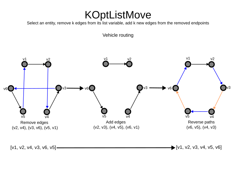
Simplest configuration:
<kOptListMoveSelector/>Advanced configuration:
    <kOptListMoveSelector>
      ... <!-- Normal selector properties -->
      <minimumK>2</minimumK>
      <maximumK>4</maximumK>
    </kOptListMoveSelector>
3.2.6. Move selectors for chained variables
TailChainSwapMoveSelector or 2-opt
A tailChain is a set of planning entities with a chained planning variable which form the last part of a chain.
The tailChainSwapMove selects a tail chain and swaps it with the tail chain of another planning value (in a different or the same anchor chain). If the targeted planning value, doesn’t have a tail chain, it swaps with nothing (resulting in a change like move). If it occurs within the same anchor chain, a partial chain reverse occurs.
In academic papers, this is often called a 2-opt move.
Simplest configuration:
<tailChainSwapMoveSelector/>Advanced configuration:
    <tailChainSwapMoveSelector>
      ... <!-- Normal selector properties -->
      <entitySelector>
        <entityClass>...Customer</entityClass>
        ...
      </entitySelector>
      <valueSelector variableName="previousStandstill">
        ...
      </valueSelector>
    </tailChainSwapMoveSelector>
The entitySelector selects the start of the tail chain that is being moved.
The valueSelector selects to where that tail chain is moved.
If it has a tail chain itself, that is moved to the location of the original tail chain.
It uses a valueSelector instead of a secondaryEntitySelector
to be able
to include all possible 2opt moves (such as moving to the end of a tail)
and to work correctly with nearby selection
(because of asymmetric distances and also swapped entity distance gives an incorrect selection probability).
|
Although |
This move selector does not support phase or solver caching.
SubChainChangeMoveSelector
A subChain is a set of planning entities with a chained planning variable which form part of a chain.
The subChainChangeMoveSelector selects a subChain and moves it to another place (in a different or the same anchor chain).
Simplest configuration:
<subChainChangeMoveSelector/>Advanced configuration:
    <subChainChangeMoveSelector>
      ... <!-- Normal selector properties -->
      <entityClass>...Customer</entityClass>
      <subChainSelector>
        <valueSelector variableName="previousStandstill">
          ...
        </valueSelector>
        <minimumSubChainSize>2</minimumSubChainSize>
        <maximumSubChainSize>40</maximumSubChainSize>
      </subChainSelector>
      <valueSelector variableName="previousStandstill">
        ...
      </valueSelector>
      <selectReversingMoveToo>true</selectReversingMoveToo>
    </subChainChangeMoveSelector>
The subChainSelector selects a number of entities, no less than minimumSubChainSize (defaults to 1) and no more than maximumSubChainSize (defaults to infinity).
|
If Furthermore, in a |
The selectReversingMoveToo property (defaults to true) enables selecting the reverse of every subchain too.
This move selector does not support phase or solver caching and step caching scales badly memory wise.
SubChainSwapMoveSelector
The subChainSwapMoveSelector selects two different subChains and moves them to another place in a different or the same anchor chain.
Simplest configuration:
<subChainSwapMoveSelector/>Advanced configuration:
    <subChainSwapMoveSelector>
      ... <!-- Normal selector properties -->
      <entityClass>...Customer</entityClass>
      <subChainSelector>
        <valueSelector variableName="previousStandstill">
          ...
        </valueSelector>
        <minimumSubChainSize>2</minimumSubChainSize>
        <maximumSubChainSize>40</maximumSubChainSize>
      </subChainSelector>
      <secondarySubChainSelector>
        <valueSelector variableName="previousStandstill">
          ...
        </valueSelector>
        <minimumSubChainSize>2</minimumSubChainSize>
        <maximumSubChainSize>40</maximumSubChainSize>
      </secondarySubChainSelector>
      <selectReversingMoveToo>true</selectReversingMoveToo>
    </subChainSwapMoveSelector>
The secondarySubChainSelector is rarely needed: if it is not specified, entities from the same subChainSelector are swapped.
The other properties are explained in subChainChangeMoveSelector. This move selector does not support phase or solver caching and step caching scales badly memory wise.
3.3. Combining multiple MoveSelectors
3.3.1. unionMoveSelector
A unionMoveSelector selects a Move by selecting one of its MoveSelector children to supply the next Move.
Simplest configuration:
    <unionMoveSelector>
      <...MoveSelector/>
      <...MoveSelector/>
      <...MoveSelector/>
      ...
    </unionMoveSelector>
Advanced configuration:
    <unionMoveSelector>
      ... <!-- Normal selector properties -->
      <changeMoveSelector>
        <fixedProbabilityWeight>...</fixedProbabilityWeight>
        ...
      </changeMoveSelector>
      <swapMoveSelector>
        <fixedProbabilityWeight>...</fixedProbabilityWeight>
        ...
      </swapMoveSelector>
      <...MoveSelector>
        <fixedProbabilityWeight>...</fixedProbabilityWeight>
        ...
      </...MoveSelector>
      ...
      <selectorProbabilityWeightFactoryClass>...ProbabilityWeightFactory</selectorProbabilityWeightFactoryClass>
    </unionMoveSelector>
The selectorProbabilityWeightFactory determines in selectionOrder RANDOM how often a MoveSelector child is selected to supply the next Move.
By default, each MoveSelector child has the same chance of being selected.
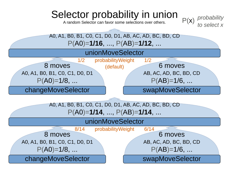
Change the fixedProbabilityWeight of such a child to select it more often.
For example, the unionMoveSelector can return a SwapMove twice as often as a ChangeMove:
    <unionMoveSelector>
      <changeMoveSelector>
        <fixedProbabilityWeight>1.0</fixedProbabilityWeight>
        ...
      </changeMoveSelector>
      <swapMoveSelector>
        <fixedProbabilityWeight>2.0</fixedProbabilityWeight>
        ...
      </swapMoveSelector>
    </unionMoveSelector>
The number of possible ChangeMoves is very different from the number of possible SwapMoves and furthermore it’s problem dependent.
To give each individual Move the same selection chance (as opposed to each MoveSelector), use the FairSelectorProbabilityWeightFactory:
    <unionMoveSelector>
      <changeMoveSelector/>
      <swapMoveSelector/>
      <selectorProbabilityWeightFactoryClass>ai.timefold.solver.core.impl.heuristic.selector.common.decorator.FairSelectorProbabilityWeightFactory</selectorProbabilityWeightFactoryClass>
    </unionMoveSelector>
3.3.2. cartesianProductMoveSelector
A cartesianProductMoveSelector selects a new CompositeMove.
It builds that CompositeMove by selecting one Move per MoveSelector child and adding it to the CompositeMove.
Simplest configuration:
    <cartesianProductMoveSelector>
      <...MoveSelector/>
      <...MoveSelector/>
      <...MoveSelector/>
      ...
    </cartesianProductMoveSelector>
Advanced configuration:
    <cartesianProductMoveSelector>
      ... <!-- Normal selector properties -->
      <changeMoveSelector>
        ...
      </changeMoveSelector>
      <swapMoveSelector>
        ...
      </swapMoveSelector>
      <...MoveSelector>
        ...
      </...MoveSelector>
      ...
      <ignoreEmptyChildIterators>true</ignoreEmptyChildIterators>
    </cartesianProductMoveSelector>
The ignoreEmptyChildIterators property (true by default) will ignore every empty childMoveSelector to avoid returning no moves.
For example: a cartesian product of changeMoveSelector A and B, for which B is empty (because all it’s entities are pinned) returns no move if ignoreEmptyChildIterators is false and the moves of A if ignoreEmptyChildIterators is true.
To enforce that two child selectors use the same entity or value efficiently, use mimic selection, not move filtering.
3.4. EntitySelector
Simplest configuration:
<entitySelector/>Advanced configuration:
      <entitySelector>
        ... <!-- Normal selector properties -->
        <entityClass>org.acme.vehiclerouting.domain.Vehicle</entityClass>
      </entitySelector>
The entityClass property is only required if it cannot be deduced automatically because there are multiple entity classes.
3.5. ValueSelector
Simplest configuration:
<valueSelector/>Advanced configuration:
      <valueSelector variableName="room">
        ... <!-- Normal selector properties -->
      </valueSelector>
The variableName property is only required if it cannot be deduced automatically because there are multiple variables (for the related entity class).
In exotic Construction Heuristic configurations, the entityClass from the EntitySelector sometimes needs to be downcasted, which can be done with the property downcastEntityClass:
      <valueSelector variableName="period">
        <downcastEntityClass>...LeadingExam</downcastEntityClass>
      </valueSelector>
If a selected entity cannot be downcasted, the ValueSelector is empty for that entity.
3.6. General Selector features
3.6.1. CacheType: create moves ahead of time or just in time
A Selector's cacheType determines when a selection (such as a Move, an entity, a value, …)
is created and how long it lives.
Almost every Selector supports setting a cacheType:
    <changeMoveSelector>
      <cacheType>PHASE</cacheType>
      ...
    </changeMoveSelector>
The following cacheTypes are supported:
-
JUST_IN_TIME(default, recommended): Not cached. Construct each selection (Move, …) just before it’s used. This scales up well in memory footprint. -
STEP: Cached. Create each selection (Move, …) at the beginning of a step and cache them in a list for the remainder of the step. This scales up badly in memory footprint. -
PHASE: Cached. Create each selection (Move, …) at the beginning of a solver phase and cache them in a list for the remainder of the phase. Some selections cannot be phase cached because the list changes every step. This scales up badly in memory footprint, but has a slight performance gain. -
SOLVER: Cached. Create each selection (Move, …) at the beginning of aSolverand cache them in a list for the remainder of theSolver. Some selections cannot be solver cached because the list changes every step. This scales up badly in memory footprint, but has a slight performance gain.
A cacheType can be set on composite selectors too:
    <unionMoveSelector>
      <cacheType>PHASE</cacheType>
      <changeMoveSelector/>
      <swapMoveSelector/>
      ...
    </unionMoveSelector>
Nested selectors of a cached selector cannot be configured to be cached themselves, unless it’s a higher cacheType.
For example: a STEP cached unionMoveSelector can contain a PHASE cached changeMoveSelector,
but it cannot contain a STEP cached changeMoveSelector.
3.6.2. SelectionOrder: original, sorted, random, shuffled, or probabilistic
A Selector's selectionOrder determines the order in which the selections (such as Moves, entities, values, …) are iterated.
An optimization algorithm will usually only iterate through a subset of its MoveSelector's selections, starting from the start, so the selectionOrder is critical to decide which Moves are actually evaluated.
Almost every Selector supports setting a selectionOrder:
    <changeMoveSelector>
      ...
      <selectionOrder>RANDOM</selectionOrder>
      ...
    </changeMoveSelector>
The following selectionOrders are supported:
-
ORIGINAL: Select the selections (Moves, entities, values, …) in default order. Each selection will be selected only once.-
For example: A0, A1, A2, A3, …, B0, B1, B2, B3, …, C0, C1, C2, C3, …
-
-
SORTED: Select the selections (
Moves, entities, values, …) in sorted order. Each selection will be selected only once. RequirescacheType >= STEP. Mostly used on anentitySelectororvalueSelectorfor construction heuristics. See sorted selection.-
For example: A0, B0, C0, …, A2, B2, C2, …, A1, B1, C1, …
-
-
RANDOM (default): Select the selections (
Moves, entities, values, …) in non-shuffled random order. A selection might be selected multiple times. This scales up well in performance because it does not require caching.-
For example: C2, A3, B1, C2, A0, C0, …
-
-
SHUFFLED: Select the selections (
Moves, entities, values, …) in shuffled random order. Each selection will be selected only once. RequirescacheType >= STEP. This scales up badly in performance, not just because it requires caching, but also because a random number is generated for each element, even if it’s not selected (which is the grand majority when scaling up).-
For example: C2, A3, B1, A0, C0, …
-
-
PROBABILISTIC: Select the selections (
Moves, entities, values, …) in random order, based on the selection probability of each element. A selection with a higher probability has a higher chance to be selected than elements with a lower probability. A selection might be selected multiple times. RequirescacheType >= STEP. Mostly used on anentitySelectororvalueSelector. See probabilistic selection.-
For example: B1, B1, A1, B2, B1, C2, B1, B1, …
-
A selectionOrder can be set on composite selectors too.
|
When a |
3.6.3. Recommended combinations of CacheType and SelectionOrder
Just in time random selection (default)
This combination is great for big use cases (10 000 entities or more), as it scales up well in memory footprint and performance.
Other combinations are often not even viable on such sizes.
It works for smaller use cases too, so it’s a good way to start out.
It’s the default, so this explicit configuration of cacheType and selectionOrder is actually obsolete:
    <unionMoveSelector>
      <cacheType>JUST_IN_TIME</cacheType>
      <selectionOrder>RANDOM</selectionOrder>

      <changeMoveSelector/>
      <swapMoveSelector/>
    </unionMoveSelector>
Here’s how it works.
When Iterator<Move>.next() is called, a child MoveSelector is randomly selected (1), which creates a random Move (2, 3, 4) and is then returned (5):
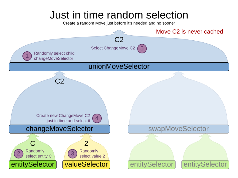
Notice that it never creates a list of Moves and it generates random numbers only for Moves that are actually selected.
Cached shuffled selection
This combination often wins for small use cases (1000 entities or less). Beyond that size, it scales up badly in memory footprint and performance.
    <unionMoveSelector>
      <cacheType>PHASE</cacheType>
      <selectionOrder>SHUFFLED</selectionOrder>

      <changeMoveSelector/>
      <swapMoveSelector/>
    </unionMoveSelector>
Here’s how it works: At the start of the phase (or step depending on the cacheType), all moves are created (1) and cached (2). When MoveSelector.iterator() is called, the moves are shuffled (3). When Iterator<Move>.next() is called, the next element in the shuffled list is returned (4):
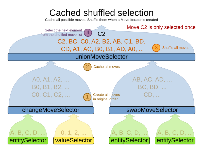
Notice that each Move will only be selected once, even though they are selected in random order.
Use cacheType PHASE if none of the (possibly nested) Selectors require STEP.
Otherwise, do something like this:
    <unionMoveSelector>
      <cacheType>STEP</cacheType>
      <selectionOrder>SHUFFLED</selectionOrder>

      <changeMoveSelector>
        <cacheType>PHASE</cacheType>
      </changeMoveSelector>
      <swapMoveSelector>
        <cacheType>PHASE</cacheType>
      </swapMoveSelector>
      <pillarSwapMoveSelector/><!-- Does not support cacheType PHASE -->
    </unionMoveSelector>
Cached random selection
This combination is often a worthy competitor for medium use cases, especially with fast stepping optimization algorithms (such as Simulated Annealing). Unlike cached shuffled selection, it doesn’t waste time shuffling the moves list at the beginning of every step.
<unionMoveSelector>
<cacheType>PHASE</cacheType>
<selectionOrder>RANDOM</selectionOrder>
<changeMoveSelector/>
<swapMoveSelector/>
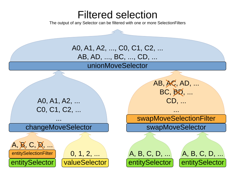
</unionMoveSelector>3.6.4. Filtered selection
There can be certain moves that you don’t want to select, because:
-
The move is pointless and would only waste CPU time. For example, swapping two lectures of the same course will result in the same score and the same schedule, because all lectures of one course are interchangeable (same teacher, same students, same topic).
-
Doing the move would break a built-in hard constraint, so the solution would be infeasible but the score function doesn’t check built-in hard constraints for performance reasons. For example, don’t change a gym lecture to a room which is not a gym room. It’s usually better to not use move filtering for such cases, because it allows the metaheuristics to temporarily break hard constraints to escape local optima.
Any built-in hard constraint must probably be filtered on every move type of every solver phase. For example if it filters the change move of Local Search, it must also filter the swap move that swaps the room of a gym lecture with another lecture for which the other lecture’s original room isn’t a gym room. Furthermore, it must also filter the change moves of the Construction Heuristics (which requires an advanced configuration).
If a move is unaccepted by the filter, it’s not executed and the score isn’t calculated.
Filtering uses the interface SelectionFilter:
public interface SelectionFilter<Solution_, T> {

    boolean accept(ScoreDirector<Solution_> scoreDirector, T selection);

}
Implement the accept method to return false on a discarded selection (see below).
Filtered selection can happen on any Selector in the selector tree, including any MoveSelector, EntitySelector
or ValueSelector.
It works with any cacheType and selectionOrder.
|
Apply the filter on the lowest level possible. In most cases, you’ll need to know both the entity and the value involved so you’ll have to apply it on the move selector. |
|
|
Filtered move selection
Unaccepted moves will not be selected and will therefore never have their doMove() method called:
public class DifferentCourseSwapMoveFilter implements SelectionFilter<CourseSchedule, SwapMove> {

    @Override
    public boolean accept(ScoreDirector<CourseSchedule> scoreDirector, SwapMove move) {
        Lecture leftLecture = (Lecture) move.getLeftEntity();
        Lecture rightLecture = (Lecture) move.getRightEntity();
        return !leftLecture.getCourse().equals(rightLecture.getCourse());
    }

}
Configure the filterClass on every targeted moveSelector
(potentially both in the Local Search and the Construction Heuristics if it filters ChangeMoves):
    <swapMoveSelector>
      <filterClass>...DifferentCourseSwapMoveFilter</filterClass>
    </swapMoveSelector>
Filtered entity selection
Unaccepted entities will not be selected and will therefore never be used to create a move.
public class LongLectureSelectionFilter implements SelectionFilter<CourseSchedule, Lecture> {

    @Override
    public boolean accept(ScoreDirector<CourseSchedule> scoreDirector, Lecture lecture) {
        return lecture.isLong();
    }

}
Configure the filterClass on every targeted entitySelector (potentially both in the Local Search and the Construction Heuristics):
    <changeMoveSelector>
      <entitySelector>
        <filterClass>...LongLectureSelectionFilter</filterClass>
      </entitySelector>
    </changeMoveSelector>
If that filter should apply on all entities, configure it as a global pinningFilter instead.
Filtered value selection
Unaccepted values will not be selected and will therefore never be used to create a move.
public class LongPeriodSelectionFilter implements SelectionFilter<CourseSchedule, Period> {

    @Override
    public boolean accept(ScoreDirector<CourseSchedule> scoreDirector, Period period) {
        return period();
    }

}
Configure the filterClass on every targeted valueSelector (potentially both in the Local Search and the Construction Heuristics):
    <changeMoveSelector>
      <valueSelector>
        <filterClass>...LongPeriodSelectionFilter</filterClass>
      </valueSelector>
    </changeMoveSelector>
3.6.5. Sorted selection
Sorted selection can happen on any Selector in the selector tree, including any MoveSelector, EntitySelector or ValueSelector.
It does not work with cacheType JUST_IN_TIME and it only works with selectionOrder SORTED.
It’s mostly used in construction heuristics.
|
If the chosen construction heuristic implies sorting, for example |
Sorted selection by SorterManner
Some Selector types implement a SorterManner out of the box:
-
EntitySelectorsupports:-
DECREASING_DIFFICULTY: Sorts the planning entities according to decreasing planning entity difficulty. Requires that planning entity difficulty is annotated on the domain model.<entitySelector> <cacheType>PHASE</cacheType> <selectionOrder>SORTED</selectionOrder> <sorterManner>DECREASING_DIFFICULTY</sorterManner> </entitySelector>
-
-
ValueSelectorsupports:-
INCREASING_STRENGTH: Sorts the planning values according to increasing planning value strength. Requires that planning value strength is annotated on the domain model.<valueSelector> <cacheType>PHASE</cacheType> <selectionOrder>SORTED</selectionOrder> <sorterManner>INCREASING_STRENGTH</sorterManner> </valueSelector>
-
Sorted selection by Comparator
An easy way to sort a Selector is with a plain old Comparator:
public class VisitDifficultyComparator implements Comparator<Visit> {
public int compare(Visit a, Visit b) {
return new CompareToBuilder()
.append(a.getServiceDuration(), b.getServiceDuration())
.append(a.getId(), b.getId())
.toComparison();
}
}You’ll also need to configure it (unless it’s annotated on the domain model and automatically applied by the optimization algorithm):
<entitySelector>
<cacheType>PHASE</cacheType>
<selectionOrder>SORTED</selectionOrder>
<sorterComparatorClass>...VisitDifficultyComparator</sorterComparatorClass>
<sorterOrder>DESCENDING</sorterOrder>
</entitySelector>|
|
Sorted selection by SelectionSorterWeightFactory
If you need the entire solution to sort a Selector, use a SelectionSorterWeightFactory instead:
public interface SelectionSorterWeightFactory<Solution_, T> {
Comparable createSorterWeight(Solution_ solution, T selection);
}You’ll also need to configure it (unless it’s annotated on the domain model and automatically applied by the optimization algorithm):
<entitySelector>
<cacheType>PHASE</cacheType>
<selectionOrder>SORTED</selectionOrder>
<sorterWeightFactoryClass>...MyDifficultyWeightFactory</sorterWeightFactoryClass>
<sorterOrder>DESCENDING</sorterOrder>
</entitySelector>|
|
Sorted selection by SelectionSorter
Alternatively, you can also use the interface SelectionSorter directly:
public interface SelectionSorter<Solution_, T> {
void sort(ScoreDirector<Solution_> scoreDirector, List<T> selectionList);
} <entitySelector>
<cacheType>PHASE</cacheType>
<selectionOrder>SORTED</selectionOrder>
<sorterClass>...MyEntitySorter</sorterClass>
</entitySelector>|
|
3.6.6. Probabilistic selection
Probabilistic selection can happen on any Selector in the selector tree, including any MoveSelector, EntitySelector or ValueSelector.
It does not work with cacheType JUST_IN_TIME and it only works with selectionOrder PROBABILISTIC.

Each selection has a probabilityWeight, which determines the chance that selection will be selected:
public interface SelectionProbabilityWeightFactory<Solution_, T> {
double createProbabilityWeight(ScoreDirector<Solution_> scoreDirector, T selection);
} <entitySelector>
<cacheType>PHASE</cacheType>
<selectionOrder>PROBABILISTIC</selectionOrder>
<probabilityWeightFactoryClass>...MyEntityProbabilityWeightFactoryClass</probabilityWeightFactoryClass>
</entitySelector>Assume the following entities: lesson A (probabilityWeight 2.0), lesson B (probabilityWeight 0.5) and lesson C (probabilityWeight 0.5). Then lesson A will be selected four times more than B and C.
|
|
3.6.7. Limited selection
Selecting all possible moves sometimes does not scale well enough, especially for construction heuristics, which don’t support acceptedCountLimit).
To limit the number of selected selection per step, apply a selectedCountLimit on the selector:
<changeMoveSelector>
<selectedCountLimit>100</selectedCountLimit>
</changeMoveSelector>|
To scale Local Search,
setting acceptedCountLimit is usually better than using |
3.6.8. Mimic selection (record/replay)
During mimic selection, one normal selector records its selection and one or multiple other special selectors replay that selection. The recording selector acts as a normal selector and supports all other configuration properties. A replaying selector mimics the recording selection and supports no other configuration properties.
The recording selector needs an id.
A replaying selector must reference a recorder’s id with a mimicSelectorRef:
<cartesianProductMoveSelector>
<changeMoveSelector>
<entitySelector id="entitySelector"/>
<valueSelector variableName="period"/>
</changeMoveSelector>
<changeMoveSelector>
<entitySelector mimicSelectorRef="entitySelector"/>
<valueSelector variableName="room"/>
</changeMoveSelector>
</cartesianProductMoveSelector>Mimic selection is useful to create a composite move from two moves that affect the same entity.
3.6.9. Nearby selection
|
Nearby selection is a commercial feature of Timefold Solver Enterprise Edition. It is not open source, and it is free for development use only. Learn more about Timefold. |
Read about nearby selection in the Nearby selection section of the Enterprise Edition manual.
3.7. Custom moves
3.7.1. Which move types might be missing in my implementation?
To determine which move types might be missing in your implementation, run a Benchmarker for a short amount of time and configure it to write the best solutions to disk. Take a look at such a best solution: it will likely be a local optima. Try to figure out if there’s a move that could get out of that local optima faster.
If you find one, implement that coarse-grained move, mix it with the existing moves and benchmark it against the previous configurations to see if you want to keep it.
3.7.2. Custom moves introduction
Instead of using the generic Moves (such as ChangeMove) you can also implement your own Move.
Generic and custom MoveSelectors can be combined as desired.
A custom Move can be tailored to work to the advantage of your constraints.
For example, in examination scheduling, changing the period of an exam A
would also change the period of all the other exams that need to coincide with exam A.
A custom Move is far more work to implement and much harder to avoid bugs than a generic Move.
After implementing a custom Move, turn on environmentMode TRACED_FULL_ASSERT to check for score corruptions.
3.7.3. The Move interface
All moves implement the Move interface:
public interface Move<Solution_> {
boolean isMoveDoable(ScoreDirector<Solution_> scoreDirector);
Move<Solution_> doMove(ScoreDirector<Solution_> scoreDirector);
...
}To implement a custom move, it’s recommended to extend AbstractMove instead implementing Move directly.
Timefold Solver calls AbstractMove.doMove(ScoreDirector), which calls doMoveOnGenuineVariables(ScoreDirector).
For example, in school timetabling, this move changes one lesson to another timeslot:
public class TimeslotChangeMove extends AbstractMove<Timetable> {
private Lesson lesson;
private Timeslot toTimeslot;
public CloudComputerChangeMove(Lesson lesson, Timeslot toTimeslot) {
this.lesson = lesson;
this.toTimeslot = toTimeslot;
}
@Override
protected void doMoveOnGenuineVariables(ScoreDirector<Timetable> scoreDirector) {
scoreDirector.beforeVariableChanged(lesson, "timeslot");
lesson.setTimeslot(toTimeslot);
scoreDirector.afterVariableChanged(lesson, "timeslot");
}
// ...
}The implementation must notify the ScoreDirector of any changes it makes to planning entity’s variables:
Call the scoreDirector.beforeVariableChanged(Object, String) and scoreDirector.afterVariableChanged(Object, String)
methods directly before and after modifying an entity’s planning variable.
The example move above is a fine-grained move because it changes only one planning variable. On the other hand, a coarse-grained move changes multiple entities or multiple planning variables in a single move, usually to avoid breaking hard constraints by making multiple related changes at once. For example, a swap move is really just two change moves, but it keeps those two changes together.
|
A |
Timefold Solver automatically filters out non doable moves by calling the isMoveDoable(ScoreDirector) method on each selected move.
A non doable move is:
-
A move that changes nothing on the current solution. For example, moving lesson
L1from timeslotXto timeslotXis not doable, because it is already there. -
A move that is impossible to do on the current solution. For example, moving lesson
L1to timeslotQ(whenQisn’t in the list of lessons) is not doable because it would assign a planning value that’s not inside the planning variable’s value range.
In the school timetabling example, a move which assigns a lesson to the timeslot it’s already assigned to is not doable:
@Override
public boolean isMoveDoable(ScoreDirector<Timetable> scoreDirector) {
return !Objects.equals(lesson.getTimeslot(), toTimeslot);
}We don’t need to check if toTimeslot is in the value range,
because we only generate moves for which that is the case.
A move that is currently not doable can become doable when the working solution changes in a later step,
otherwise we probably shouldn’t have created it in the first place.
Each move has an undo move: a move (normally of the same type) which does the exact opposite.
In the cloud balancing example the undo move of L1 {X → Y} is the move L1 {Y → X}.
The undo move of a move is created when the Move is being done on the current solution,
before the genuine variables change:
@Override
public TimeslotChangeMove createUndoMove(ScoreDirector<Timetable> scoreDirector) {
return new TimeslotChangeMove(lesson, lesson.getTimeslot());
}Notice that if L1 would have already been moved to Y, the undo move would create the move L1 {Y → Y},
instead of the move L1 {Y → X}.
A solver phase might do and undo the same Move more than once.
In fact, many solver phases will iteratively do and undo a number of moves to evaluate them,
before selecting one of those and doing that move again (without undoing it the last time).
Always implement the toString() method to keep Timefold Solver’s logs readable.
Keep it non-verbose and make it consistent with the generic moves:
public String toString() {
return lesson + " {" + lesson.getTimeslot() + " -> " + toTimeslot + "}";
}Optionally, implement the getSimpleMoveTypeDescription() method to support
picked move statistics:
@Override
public String getSimpleMoveTypeDescription() {
return "TimeslotChangeMove(Lesson.timeslot)";
}Custom move: rebase()
For multi-threaded incremental solving,
the custom move must implement the rebase() method:
@Override
public TimeslotChangeMove rebase(ScoreDirector<Timetable> destinationScoreDirector) {
return new TimeslotChangeMove(destinationScoreDirector.lookUpWorkingObject(lesson),
destinationScoreDirector.lookUpWorkingObject(toTimeslot));
}Rebasing a move takes a move generated from one working solution and creates a new move that does the same change as the original move, but rewired as if it was generated from the destination working solution. This allows multi-threaded solving to migrate moves from one thread to another.
The lookUpWorkingObject() method translates a planning entity instance or problem fact instance
from one working solution to that of the destination’s working solution.
Internally it often uses a mapping technique based on the planning ID.
To rebase lists or arrays in bulk, use rebaseList() and rebaseArray() on AbstractMove.
Custom move: getPlanningEntities() and getPlanningValues()
A custom move should also implement the getPlanningEntities() and getPlanningValues() methods.
Those are used by entity tabu and value tabu respectively.
They are called after the Move has already been done.
@Override
public Collection<? extends Object> getPlanningEntities() {
return Collections.singletonList(lesson);
}
@Override
public Collection<? extends Object> getPlanningValues() {
return Collections.singletonList(toTimeslot);
}If the Move changes multiple planning entities, such as in a swap move,
return all of them in getPlanningEntities()
and return all their values (to which they are changing) in getPlanningValues().
@Override
public Collection<? extends Object> getPlanningEntities() {
return Arrays.asList(leftLesson, rightLesson);
}
@Override
public Collection<? extends Object> getPlanningValues() {
return Arrays.asList(leftLesson.getTimeslot(), rightLesson.getTimeslot());
}Custom move: equals() and hashCode()
A Move must implement the equals() and hashCode() methods for move tabu.
Two moves which make the same change on a solution, should be equal ideally.
@Override
public boolean equals(Object o) {
return o instanceof TimeslotChangeMove other
&& lesson.equals(other.lesson)
&& toTimeslot.equals(other.toTimeslot);
}
@Override
public int hashCode() {
return new HashCodeBuilder()
.append(lesson)
.append(toTimeslot)
.toHashCode();
}Notice that it checks if the other move is an instance of the same move type.
This instanceof check is important because a move are compared to a move of another move type.
For example a ChangeMove and SwapMove are compared.
3.7.4. Generating custom moves
Now, let’s generate instances of this custom Move class.
There are 2 ways:
MoveListFactory: the easy way to generate custom moves
The easiest way to generate custom moves is by implementing the interface MoveListFactory:
public interface MoveListFactory<Solution_> {
List<Move> createMoveList(Solution_ solution);
}Simple configuration (which can be nested in a unionMoveSelector just like any other MoveSelector):
<moveListFactory>
<moveListFactoryClass>...MyMoveFactory</moveListFactoryClass>
</moveListFactory>Advanced configuration:
<moveListFactory>
... <!-- Normal moveSelector properties -->
<moveListFactoryClass>...MyMoveFactory</moveListFactoryClass>
<moveListFactoryCustomProperties>
...<!-- Custom properties -->
</moveListFactoryCustomProperties>
</moveListFactory>Because the MoveListFactory generates all moves at once in a List<Move>,
it does not support cacheType JUST_IN_TIME.
Therefore, moveListFactory uses cacheType STEP by default and it scales badly.
To configure values of a MoveListFactory dynamically in the solver configuration
(so the Benchmarker can tweak those parameters),
add the moveListFactoryCustomProperties element and use custom properties.
|
A custom |
MoveIteratorFactory: generate Custom moves just in time
Use this advanced form to generate custom moves Just In Time
by implementing the MoveIteratorFactory interface:
public interface MoveIteratorFactory<Solution_> {
long getSize(ScoreDirector<Solution_> scoreDirector);
Iterator<Move> createOriginalMoveIterator(ScoreDirector<Solution_> scoreDirector);
Iterator<Move> createRandomMoveIterator(ScoreDirector<Solution_> scoreDirector, Random workingRandom);
}The getSize() method must return an estimation of the size.
It doesn’t need to be correct, but it’s better too big than too small.
The createOriginalMoveIterator method is called if the selectionOrder is ORIGINAL or if it is cached.
The createRandomMoveIterator method is called for selectionOrder RANDOM combined with cacheType JUST_IN_TIME.
|
Don’t create a collection (array, list, set or map) of |
For example:
public class PossibleAssignmentsOnlyMoveIteratorFactory implements MoveIteratorFactory<MyPlanningSolution, MyChangeMove> {
@Override
public long getSize(ScoreDirector<MyPlanningSolution> scoreDirector) {
// In this case, we return the exact size, but an estimate can be used
// if it too expensive to calculate or unknown
long totalSize = 0L;
var solution = scoreDirector.getWorkingSolution();
for (MyEntity entity : solution.getEntities()) {
for (MyPlanningValue value : solution.getValues()) {
if (entity.canBeAssigned(value)) {
totalSize++;
}
}
}
return totalSize;
}
@Override
public Iterator<MyChangeMove> createOriginalMoveIterator(ScoreDirector<MyPlanningSolution> scoreDirector) {
// Only needed if selectionOrder is ORIGINAL or if it is cached
var solution = scoreDirector.getWorkingSolution();
var entities = solution.getEntities();
var values = solution.getValues();
// Assumes each entity has at least one assignable value
var firstEntityIndex = 0;
var firstValueIndex = 0;
while (!entities.get(firstEntityIndex).canBeAssigned(values.get(firstValueIndex))) {
firstValueIndex++;
}
return new Iterator<>() {
int nextEntityIndex = firstEntityIndex;
int nextValueIndex = firstValueIndex;
@Override
public boolean hasNext() {
return nextEntityIndex < entities.size();
}
@Override
public MyChangeMove next() {
var selectedEntity = entities.get(nextEntityIndex);
var selectedValue = values.get(nextValueIndex);
nextValueIndex++;
while (nextValueIndex < values.size() && !selectedEntity.canBeAssigned(values.get(nextValueIndex))) {
nextValueIndex++;
}
if (nextValueIndex >= values.size()) {
// value list exhausted, go to next entity
nextEntityIndex++;
if (nextEntityIndex < entities.size()) {
nextValueIndex = 0;
while (nextValueIndex < values.size() && !entities.get(nextEntityIndex).canBeAssigned(values.get(nextValueIndex))) {
// Assumes each entity has at least one assignable value
nextValueIndex++;
}
}
}
return new MyChangeMove(selectedEntity, selectedValue);
}
};
}
@Override
public Iterator<MyChangeMove> createRandomMoveIterator(ScoreDirector<MyPlanningSolution> scoreDirector,
Random workingRandom) {
// Not needed if selectionOrder is ORIGINAL or if it is cached
var solution = scoreDirector.getWorkingSolution();
var entities = solution.getEntities();
var values = solution.getValues();
return new Iterator<>() {
@Override
public boolean hasNext() {
return !entities.isEmpty();
}
@Override
public MyChangeMove next() {
var selectedEntity = entities.get(workingRandom.nextInt(entities.size()));
var selectedValue = values.get(workingRandom.nextInt(values.size()));
while (!selectedEntity.canBeAssigned(selectedValue)) {
// This assumes there at least one value that can be assigned to the selected entity
selectedValue = values.get(workingRandom.nextInt(values.size()));
}
return new MyChangeMove(selectedEntity, selectedValue);
}
};
}
}|
The same effect can also be accomplished using filtered selection. |
Simple configuration (which can be nested in a unionMoveSelector just like any other MoveSelector):
<moveIteratorFactory>
<moveIteratorFactoryClass>...</moveIteratorFactoryClass>
</moveIteratorFactory>Advanced configuration:
<moveIteratorFactory>
... <!-- Normal moveSelector properties -->
<moveIteratorFactoryClass>...</moveIteratorFactoryClass>
<moveIteratorFactoryCustomProperties>
...<!-- Custom properties -->
</moveIteratorFactoryCustomProperties>
</moveIteratorFactory>To configure values of a MoveIteratorFactory dynamically in the solver configuration
(so the Benchmarker can tweak those parameters),
add the moveIteratorFactoryCustomProperties element and use custom properties.
|
A custom |
4. Exhaustive search
4.1. Overview
Exhaustive Search will always find the global optimum and recognize it too. That being said, it doesn’t scale (not even beyond toy data sets) and is therefore mostly useless.
4.2. Brute force
4.2.1. Algorithm description
The Brute Force algorithm creates and evaluates every possible solution.
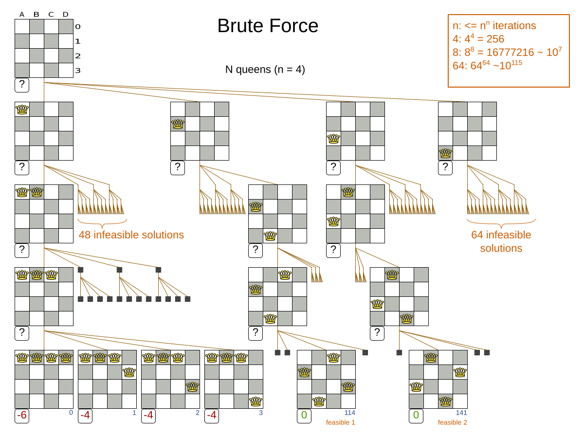
Notice that it creates a search tree that explodes exponentially as the problem size increases, so it hits a scalability wall.
|
Brute Force is mostly unusable for a real-world problem due to time limitations, as shown in scalability of Exhaustive Search. |
4.2.2. Configuration
Simplest configuration of Brute Force:
<solver xmlns="https://timefold.ai/xsd/solver" xmlns:xsi="http://www.w3.org/2001/XMLSchema-instance"
xsi:schemaLocation="https://timefold.ai/xsd/solver https://timefold.ai/xsd/solver/solver.xsd">
...
<exhaustiveSearch>
<exhaustiveSearchType>BRUTE_FORCE</exhaustiveSearchType>
</exhaustiveSearch>
</solver>4.3. Branch and bound
4.3.1. Algorithm description
Branch And Bound also explores nodes in an exponential search tree, but it investigates more promising nodes first and prunes away worthless nodes.
For each node, Branch And Bound calculates the optimistic bound: the best possible score to which that node can lead to. If the optimistic bound of a node is lower or equal to the global pessimistic bound, then it prunes away that node (including the entire branch of all its subnodes).
|
Academic papers use the term lower bound instead of optimistic bound (and the term upper bound instead of pessimistic bound), because they minimize the score. Timefold Solver maximizes the score (because it supports combining negative and positive constraints). Therefore, for clarity, it uses different terms, as it would be confusing to use the term lower bound for a bound which is always higher. |
For example: at index 14, it sets the global pessimistic bound to -2.
Because all solutions reachable from the node visited at index 11 will have a score lower or equal to -2 (the node’s optimistic bound), they can be pruned away.
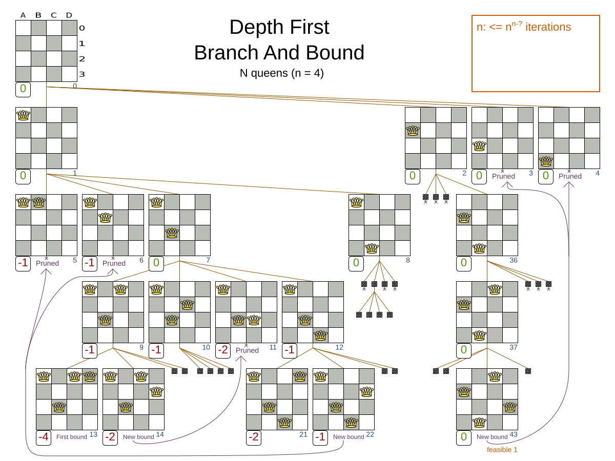
Notice that Branch And Bound (much like Brute Force) creates a search tree that explodes exponentially as the problem size increases. So it hits the same scalability wall, only a little bit later.
|
Branch And Bound is mostly unusable for a real-world problem due to time limitations, as shown in scalability of Exhaustive Search. |
4.3.2. Configuration
Simplest configuration of Branch And Bound:
<solver xmlns="https://timefold.ai/xsd/solver" xmlns:xsi="http://www.w3.org/2001/XMLSchema-instance"
xsi:schemaLocation="https://timefold.ai/xsd/solver https://timefold.ai/xsd/solver/solver.xsd">
...
<exhaustiveSearch>
<exhaustiveSearchType>BRANCH_AND_BOUND</exhaustiveSearchType>
</exhaustiveSearch>
</solver>|
For the pruning to work with the default |
Advanced configuration:
<exhaustiveSearch>
<exhaustiveSearchType>BRANCH_AND_BOUND</exhaustiveSearchType>
<nodeExplorationType>DEPTH_FIRST</nodeExplorationType>
<entitySorterManner>DECREASING_DIFFICULTY_IF_AVAILABLE</entitySorterManner>
<valueSorterManner>INCREASING_STRENGTH_IF_AVAILABLE</valueSorterManner>
</exhaustiveSearch>The nodeExplorationType options are:
-
DEPTH_FIRST(default): Explore deeper nodes first (and then a better score and then a better optimistic bound). Deeper nodes (especially leaf nodes) often improve the pessimistic bound. A better pessimistic bound allows pruning more nodes to reduce the search space.<exhaustiveSearch> <exhaustiveSearchType>BRANCH_AND_BOUND</exhaustiveSearchType> <nodeExplorationType>DEPTH_FIRST</nodeExplorationType> </exhaustiveSearch> -
BREADTH_FIRST(not recommended): Explore nodes layer by layer (and then a better score and then a better optimistic bound). Scales terribly in memory (and usually in performance too).<exhaustiveSearch> <exhaustiveSearchType>BRANCH_AND_BOUND</exhaustiveSearchType> <nodeExplorationType>BREADTH_FIRST</nodeExplorationType> </exhaustiveSearch> -
SCORE_FIRST: Explore nodes with a better score first (and then a better optimistic bound and then deeper nodes first). Might scale as terribly asBREADTH_FIRSTin some cases.<exhaustiveSearch> <exhaustiveSearchType>BRANCH_AND_BOUND</exhaustiveSearchType> <nodeExplorationType>SCORE_FIRST</nodeExplorationType> </exhaustiveSearch> -
OPTIMISTIC_BOUND_FIRST: Explore nodes with a better optimistic bound first (and then a better score and then deeper nodes first). Might scale as terribly asBREADTH_FIRSTin some cases.<exhaustiveSearch> <exhaustiveSearchType>BRANCH_AND_BOUND</exhaustiveSearchType> <nodeExplorationType>OPTIMISTIC_BOUND_FIRST</nodeExplorationType> </exhaustiveSearch>
The entitySorterManner options are:
-
DECREASING_DIFFICULTY: Initialize the more difficult planning entities first. This usually increases pruning (and therefore improves scalability). Requires the model to support planning entity difficulty comparison. -
DECREASING_DIFFICULTY_IF_AVAILABLE(default): If the model supports planning entity difficulty comparison, behave likeDECREASING_DIFFICULTY, else likeNONE. -
NONE: Initialize the planning entities in original order.
The valueSorterManner options are:
-
INCREASING_STRENGTH: Evaluate the planning values in increasing strength. Requires the model to support planning value strength comparison. -
INCREASING_STRENGTH_IF_AVAILABLE(default): If the model supports planning value strength comparison, behave likeINCREASING_STRENGTH, else likeNONE. -
DECREASING_STRENGTH: Evaluate the planning values in decreasing strength. Requires the model to support planning value strength comparison. -
DECREASING_STRENGTH_IF_AVAILABLE: If the model supports planning value strength comparison, behave likeDECREASING_STRENGTH, else likeNONE. -
NONE: Try the planning values in original order.
4.4. Scalability of exhaustive search
Exhaustive Search variants suffer from two big scalability issues:
-
They scale terribly memory wise.
-
They scale horribly performance wise.
As shown in these time spent graphs from the Benchmarker, Brute Force and Branch And Bound both hit a performance scalability wall. For example, on N queens it hits wall at a few dozen queens:
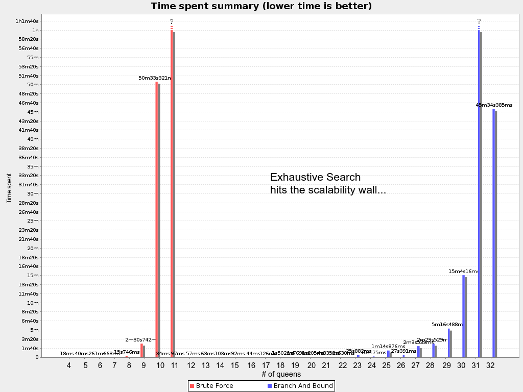
In most use cases, the wall appears out of thin air. Exhaustive Search hits this wall on small datasets already, so in production these optimizations algorithms are mostly useless. Use Construction Heuristics with Local Search instead: those can handle thousands of entities easily.
|
Throwing hardware at these scalability issues has no noticeable impact. Moore’s law cannot win against the onslaught of a few more planning entities in the dataset. |
5. Construction heuristics
5.1. Overview
A construction heuristic builds a pretty good initial solution in a finite length of time. Its solution isn’t always feasible, but it finds it fast so metaheuristics can finish the job.
Construction heuristics terminate automatically, so there’s usually no need to configure a Termination on the construction heuristic phase specifically.
5.2. First fit
5.2.1. Algorithm description
The First Fit algorithm cycles through all the planning entities (in default order), initializing one planning entity at a time. It assigns the planning entity to the best available planning value, taking the already initialized planning entities into account. It terminates when all planning entities have been initialized. It never changes a planning entity after it has been assigned.

Notice that it starts with putting Queen A into row 0 (and never moving it later),
which makes it impossible to reach the optimal solution.
Suffixing this construction heuristic with metaheuristics can remedy that.
5.2.2. Configuration
Simple configuration:
<constructionHeuristic>
<constructionHeuristicType>FIRST_FIT</constructionHeuristicType>
</constructionHeuristic>Advanced configuration:
<constructionHeuristic>
<constructionHeuristicType>FIRST_FIT</constructionHeuristicType>
<...MoveSelector/>
<...MoveSelector/>
...
</constructionHeuristic>For scaling out, see scaling construction heuristics. For a very advanced configuration, see Allocate Entity From Queue.
5.3. First fit decreasing
5.3.1. Algorithm description
Like First Fit, but assigns the more difficult planning entities first, because they are less likely to fit in the leftovers. So it sorts the planning entities on decreasing difficulty.
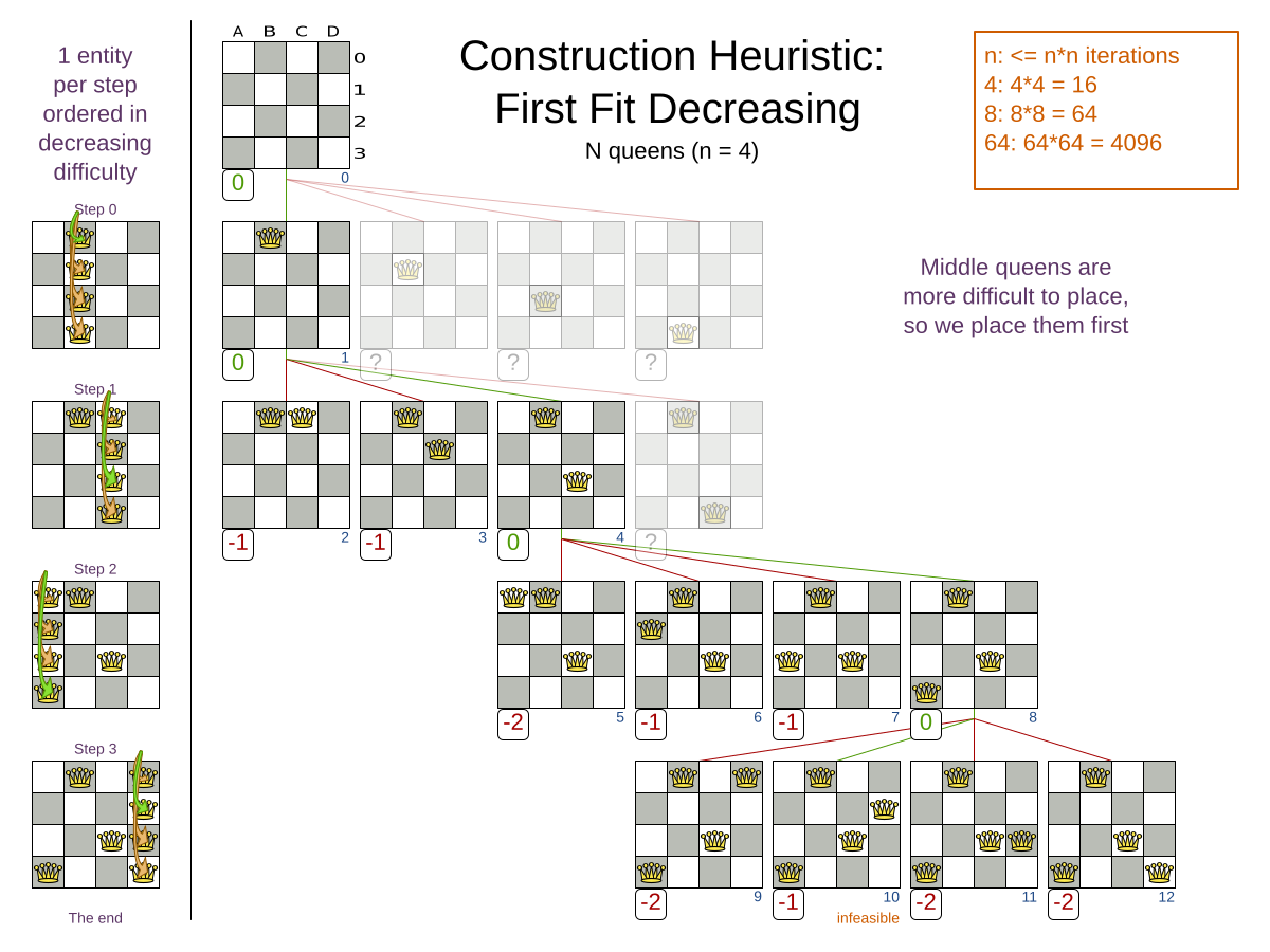
Requires the model to support planning entity difficulty comparison.
|
One would expect that this algorithm has better results than First Fit. That’s usually the case, but not always. |
5.3.2. Configuration
Simple configuration:
<constructionHeuristic>
<constructionHeuristicType>FIRST_FIT_DECREASING</constructionHeuristicType>
</constructionHeuristic>Advanced configuration:
<constructionHeuristic>
<constructionHeuristicType>FIRST_FIT_DECREASING</constructionHeuristicType>
<...MoveSelector/>
<...MoveSelector/>
...
</constructionHeuristic>For scaling out, see scaling construction heuristics. For a very advanced configuration, see Allocate Entity From Queue.
5.4. Weakest fit
5.4.1. Algorithm description
Like First Fit, but uses the weaker planning values first, because the strong planning values are more likely to be able to accommodate later planning entities. So it sorts the planning values on increasing strength.
Requires the model to support planning value strength comparison.
|
Do not presume that this algorithm has better results than First Fit. That’s often not the case. |
5.4.2. Configuration
Simple configuration:
<constructionHeuristic>
<constructionHeuristicType>WEAKEST_FIT</constructionHeuristicType>
</constructionHeuristic>Advanced configuration:
<constructionHeuristic>
<constructionHeuristicType>WEAKEST_FIT</constructionHeuristicType>
<...MoveSelector/>
<...MoveSelector/>
...
</constructionHeuristic>For scaling out, see scaling construction heuristics. For a very advanced configuration, see Allocate Entity From Queue.
5.5. Weakest fit decreasing
5.5.1. Algorithm description
Combines First Fit Decreasing and Weakest Fit. So it sorts the planning entities on decreasing difficulty and the planning values on increasing strength.
Requires the model to support planning entity difficulty comparison and planning value strength comparison.
|
Do not presume that this algorithm has better results than First Fit Decreasing. That’s often not the case. However, it is usually better than Weakest Fit. |
5.5.2. Configuration
Simple configuration:
<constructionHeuristic>
<constructionHeuristicType>WEAKEST_FIT_DECREASING</constructionHeuristicType>
</constructionHeuristic>Advanced configuration:
<constructionHeuristic>
<constructionHeuristicType>WEAKEST_FIT_DECREASING</constructionHeuristicType>
<...MoveSelector/>
<...MoveSelector/>
...
</constructionHeuristic>For scaling out, see scaling construction heuristics. For a very advanced configuration, see Allocate Entity From Queue.
5.6. Strongest fit
5.6.1. Algorithm description
Like First Fit, but uses the strong planning values first, because the strong planning values are more likely to have a lower soft cost to use. So it sorts the planning values on decreasing strength.
Requires the model to support planning value strength comparison.
|
Do not presume that this algorithm has better results than First Fit or Weakest Fit. That’s often not the case. |
5.6.2. Configuration
Simple configuration:
<constructionHeuristic>
<constructionHeuristicType>STRONGEST_FIT</constructionHeuristicType>
</constructionHeuristic>Advanced configuration:
<constructionHeuristic>
<constructionHeuristicType>STRONGEST_FIT</constructionHeuristicType>
<...MoveSelector/>
<...MoveSelector/>
...
</constructionHeuristic>For scaling out, see scaling construction heuristics. For a very advanced configuration, see Allocate Entity From Queue.
5.7. Strongest fit decreasing
5.7.1. Algorithm description
Combines First Fit Decreasing and Strongest Fit. So it sorts the planning entities on decreasing difficulty and the planning values on decreasing strength.
Requires the model to support planning entity difficulty comparison and planning value strength comparison.
|
Do not presume that this algorithm has better results than First Fit Decreasing or Weakest Fit Decreasing. That’s often not the case. However, it is usually better than Strongest Fit. |
5.7.2. Configuration
Simple configuration:
<constructionHeuristic>
<constructionHeuristicType>STRONGEST_FIT_DECREASING</constructionHeuristicType>
</constructionHeuristic>Advanced configuration:
<constructionHeuristic>
<constructionHeuristicType>STRONGEST_FIT_DECREASING</constructionHeuristicType>
<...MoveSelector/>
<...MoveSelector/>
...
</constructionHeuristic>For scaling out, see scaling construction heuristics. For a very advanced configuration, see Allocate Entity From Queue.
5.8. Allocate entity from queue
5.8.1. Algorithm description
Allocate Entity From Queue is a versatile, generic form of First Fit, First Fit Decreasing, Weakest Fit, Weakest Fit Decreasing, Strongest Fit and Strongest Fit Decreasing. It works like this:
-
Put all entities in a queue.
-
Assign the first entity (from that queue) to the best value.
-
Repeat until all entities are assigned.
5.8.2. Configuration
Simple configuration:
<constructionHeuristic>
<constructionHeuristicType>ALLOCATE_ENTITY_FROM_QUEUE</constructionHeuristicType>
</constructionHeuristic>Verbose simple configuration:
<constructionHeuristic>
<constructionHeuristicType>ALLOCATE_ENTITY_FROM_QUEUE</constructionHeuristicType>
<entitySorterManner>DECREASING_DIFFICULTY_IF_AVAILABLE</entitySorterManner>
<valueSorterManner>INCREASING_STRENGTH_IF_AVAILABLE</valueSorterManner>
</constructionHeuristic>The entitySorterManner options are:
-
DECREASING_DIFFICULTY: Initialize the more difficult planning entities first. This usually increases pruning (and therefore improves scalability). Requires the model to support planning entity difficulty comparison. -
DECREASING_DIFFICULTY_IF_AVAILABLE(default): If the model supports planning entity difficulty comparison, behave likeDECREASING_DIFFICULTY, else likeNONE. -
NONE: Initialize the planning entities in original order.
The valueSorterManner options are:
-
INCREASING_STRENGTH: Evaluate the planning values in increasing strength. Requires the model to support planning value strength comparison. -
INCREASING_STRENGTH_IF_AVAILABLE(default): If the model supports planning value strength comparison, behave likeINCREASING_STRENGTH, else likeNONE. -
DECREASING_STRENGTH: Evaluate the planning values in decreasing strength. Requires the model to support planning value strength comparison. -
DECREASING_STRENGTH_IF_AVAILABLE: If the model supports planning value strength comparison, behave likeDECREASING_STRENGTH, else likeNONE. -
NONE: Try the planning values in original order.
Advanced configuration with Weakest Fit Decreasing for a single entity class with one variable:
<constructionHeuristic>
<queuedEntityPlacer>
<entitySelector id="placerEntitySelector">
<cacheType>PHASE</cacheType>
<selectionOrder>SORTED</selectionOrder>
<sorterManner>DECREASING_DIFFICULTY</sorterManner>
</entitySelector>
<changeMoveSelector>
<entitySelector mimicSelectorRef="placerEntitySelector"/>
<valueSelector>
<cacheType>PHASE</cacheType>
<selectionOrder>SORTED</selectionOrder>
<sorterManner>INCREASING_STRENGTH</sorterManner>
</valueSelector>
</changeMoveSelector>
</queuedEntityPlacer>
</constructionHeuristic>Per step, the QueuedEntityPlacer selects one uninitialized entity from the EntitySelector
and applies the winning Move (out of all the moves for that entity generated by the MoveSelector).
The mimic selection ensures that the winning Move changes only the selected entity.
To customize the entity or value sorting, see sorted selection. For scaling out, see scaling construction heuristics.
If there are multiple planning variables, there’s one ChangeMoveSelector per planning variable,
which are either in a cartesian product or in sequential steps,
similar to the less verbose configuration.
5.8.3. Multiple entity classes
The easiest way to deal with multiple entity classes is to run a separate Construction Heuristic for each entity class:
<constructionHeuristic>
<queuedEntityPlacer>
<entitySelector id="placerEntitySelector">
<entityClass>...DogEntity</entityClass>
<cacheType>PHASE</cacheType>
</entitySelector>
<changeMoveSelector>
<entitySelector mimicSelectorRef="placerEntitySelector"/>
</changeMoveSelector>
</queuedEntityPlacer>
...
</constructionHeuristic>
<constructionHeuristic>
<queuedEntityPlacer>
<entitySelector id="placerEntitySelector">
<entityClass>...CatEntity</entityClass>
<cacheType>PHASE</cacheType>
</entitySelector>
<changeMoveSelector>
<entitySelector mimicSelectorRef="placerEntitySelector"/>
</changeMoveSelector>
</queuedEntityPlacer>
...
</constructionHeuristic>5.8.4. Pick early type
There are several pick early types for Construction Heuristics:
-
NEVER: Evaluate all the selected moves to initialize the variable(s). This is the default if the InitializingScoreTrend is notONLY_DOWN.<constructionHeuristic> ... <forager> <pickEarlyType>NEVER</pickEarlyType> </forager> </constructionHeuristic> -
FIRST_NON_DETERIORATING_SCORE: Initialize the variable(s) with the first move that doesn’t deteriorate the score, ignore the remaining selected moves. This is the default if the InitializingScoreTrend isONLY_DOWN.<constructionHeuristic> ... <forager> <pickEarlyType>FIRST_NON_DETERIORATING_SCORE</pickEarlyType> </forager> </constructionHeuristic>If there are only negative constraints, but the InitializingScoreTrend is strictly not
ONLY_DOWN, it can sometimes make sense to apply FIRST_NON_DETERIORATING_SCORE. Use the Benchmarker to decide if the score quality loss is worth the time gain. -
FIRST_FEASIBLE_SCORE: Initialize the variable(s) with the first move that has a feasible score.<constructionHeuristic> ... <forager> <pickEarlyType>FIRST_FEASIBLE_SCORE</pickEarlyType> </forager> </constructionHeuristic>If the InitializingScoreTrend is
ONLY_DOWN, useFIRST_FEASIBLE_SCORE_OR_NON_DETERIORATING_HARDinstead, because that’s faster without any disadvantages. -
FIRST_FEASIBLE_SCORE_OR_NON_DETERIORATING_HARD: Initialize the variable(s) with the first move that doesn’t deteriorate the feasibility of the score any further.<constructionHeuristic> ... <forager> <pickEarlyType>FIRST_FEASIBLE_SCORE_OR_NON_DETERIORATING_HARD</pickEarlyType> </forager> </constructionHeuristic>
5.9. Allocate to value from queue
5.9.1. Algorithm description
Allocate To Value From Queue works like this:
-
Put all values in a round-robin queue.
-
Assign the best entity to the first value (from that queue).
-
Repeat until all entities are assigned.
5.9.2. Configuration
Simple configuration:
<constructionHeuristic>
<constructionHeuristicType>ALLOCATE_TO_VALUE_FROM_QUEUE</constructionHeuristicType>
</constructionHeuristic>Verbose simple configuration:
<constructionHeuristic>
<constructionHeuristicType>ALLOCATE_TO_VALUE_FROM_QUEUE</constructionHeuristicType>
<entitySorterManner>DECREASING_DIFFICULTY_IF_AVAILABLE</entitySorterManner>
<valueSorterManner>INCREASING_STRENGTH_IF_AVAILABLE</valueSorterManner>
</constructionHeuristic>Advanced configuration for a single entity class with a single variable:
<constructionHeuristic>
<queuedValuePlacer>
<valueSelector id="placerValueSelector">
<cacheType>PHASE</cacheType>
<selectionOrder>SORTED</selectionOrder>
<sorterManner>INCREASING_STRENGTH</sorterManner>
</valueSelector>
<changeMoveSelector>
    <entitySelector>
      <cacheType>PHASE</cacheType>
      <selectionOrder>SORTED</selectionOrder>
      <sorterManner>DECREASING_DIFFICULTY</sorterManner>
    </entitySelector>
<valueSelector mimicSelectorRef="placerValueSelector"/>
</changeMoveSelector>
</queuedValuePlacer>
</constructionHeuristic>For scaling out, see scaling construction heuristics.
5.10. Cheapest insertion
5.10.1. Algorithm description
The Cheapest Insertion algorithm cycles through all the planning values for all the planning entities, initializing one planning entity at a time. It assigns a planning entity to the best available planning value (out of all the planning entities and values), taking the already initialized planning entities into account. It terminates when all planning entities have been initialized. It never changes a planning entity after it has been assigned.
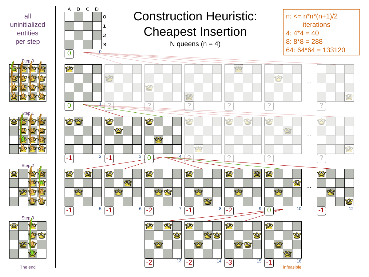
|
Cheapest Insertion scales considerably worse than First Fit, etc. |
5.10.2. Configuration
Simple configuration:
<constructionHeuristic>
<constructionHeuristicType>CHEAPEST_INSERTION</constructionHeuristicType>
</constructionHeuristic>Advanced configuration:
<constructionHeuristic>
<constructionHeuristicType>CHEAPEST_INSERTION</constructionHeuristicType>
<...MoveSelector/>
<...MoveSelector/>
...
</constructionHeuristic>For scaling out, see scaling construction heuristics. For a very advanced configuration, see Allocate from pool.
5.11. Regret insertion
5.11.1. Algorithm description
The Regret Insertion algorithm behaves like the Cheapest Insertion algorithm. It also cycles through all the planning values for all the planning entities, initializing one planning entity at a time. But instead of picking the entity-value combination with the best score, it picks the entity which has the largest score loss between its best and second best value assignment. It then assigns that entity to its best value, to avoid regretting not having done that.
5.12. Allocate from pool
5.12.1. Algorithm description
Allocate From Pool is a versatile, generic form of Cheapest Insertion and Regret Insertion. It works like this:
-
Put all entity-value combinations in a pool.
-
Assign the best entity to best value.
-
Repeat until all entities are assigned.
5.12.2. Configuration
Simple configuration:
<constructionHeuristic>
<constructionHeuristicType>ALLOCATE_FROM_POOL</constructionHeuristicType>
</constructionHeuristic>Verbose simple configuration:
<constructionHeuristic>
<constructionHeuristicType>ALLOCATE_FROM_POOL</constructionHeuristicType>
<entitySorterManner>DECREASING_DIFFICULTY_IF_AVAILABLE</entitySorterManner>
<valueSorterManner>INCREASING_STRENGTH_IF_AVAILABLE</valueSorterManner>
</constructionHeuristic>The entitySorterManner and valueSorterManner options are described in Allocate Entity From Queue.
Advanced configuration with Cheapest Insertion for a single entity class with a single variable:
<constructionHeuristic>
<pooledEntityPlacer>
<changeMoveSelector>
<entitySelector id="placerEntitySelector">
<cacheType>PHASE</cacheType>
<selectionOrder>SORTED</selectionOrder>
<sorterManner>DECREASING_DIFFICULTY</sorterManner>
</entitySelector>
    <valueSelector>
      <cacheType>PHASE</cacheType>
      <selectionOrder>SORTED</selectionOrder>
      <sorterManner>INCREASING_STRENGTH</sorterManner>
    </valueSelector>
</changeMoveSelector>
</pooledEntityPlacer>
</constructionHeuristic>Per step, the PooledEntityPlacer applies the winning Move (out of all the moves for that entity generated by the MoveSelector).
To customize the entity or value sorting,
see sorted selection.
Other Selector customization
(such as filtering
and limiting)
is supported too.
For scaling out, see scaling construction heuristics.
5.13. Scaling construction heuristics
If the Construction Heuristic takes a long time to solve and create an initial solution, there is too little time left for Local Search to reach a near optimal solution.
Ideally, a Construction Heuristic should take less than 20 seconds from scratch and less than 50 milliseconds in real-time planning, so there is plenty of time left for Local Search. If the Benchmarker proves that this is not the case, there’s a number of improvements that can be done:
5.13.1. InitializingScoreTrend shortcuts
If the InitializingScoreTrend is ONLY_DOWN, a Construction Heuristic algorithm (such as First Fit) is faster:
for an entity, it picks the first move for which the score does not deteriorate the last step score, ignoring all subsequent moves in that step.
It can take that shortcut without reducing solution quality, because a down trend guarantees that initializing any additional planning variable can only make the score the same or worse. So if a move has the same score as before the planning variable was initialized, then no other move can have a better score.
5.13.2. Scaling multiple planning variables in construction heuristics
There are two ways to deal with multiple planning variables,
depending on how their ChangeMoves are combined:
-
Cartesian product (default): All variables of the selected entity are assigned together. This usually results in a better solution quality, but it scales poorly because it tries every combination of variables. For example:
<constructionHeuristic> <constructionHeuristicType>FIRST_FIT_DECREASING</constructionHeuristicType> <cartesianProductMoveSelector> <changeMoveSelector> <valueSelector variableName="period"/> </changeMoveSelector> <changeMoveSelector> <valueSelector variableName="room"/> </changeMoveSelector> </cartesianProductMoveSelector> </constructionHeuristic> -
Sequential: One variable is assigned at a time. Scales better, at the cost of solution quality. The order of the planning variables matters. For example:
  <constructionHeuristic>
    <constructionHeuristicType>FIRST_FIT_DECREASING</constructionHeuristicType>
    <changeMoveSelector>
      <valueSelector variableName="period"/>
    </changeMoveSelector>
    <changeMoveSelector>
      <valueSelector variableName="room"/>
    </changeMoveSelector>
  </constructionHeuristic>
The second way scales better, so it can be worth to switch to it. Especially for three or more planning variables, the scaling difference is huge. For example, with three variables of 1 000 values each, a cartesian product selects 1 000 000 000 moves per entity (1 step per entity). A sequential approach only selects 3 000 moves per entity (3 steps per entity), ending the Construction Heuristic 300 000 times faster.
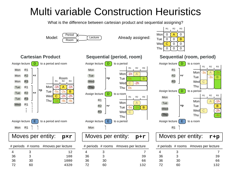
|
The order of the variables is important, especially in the sequential technique.
In the sequential example above, it’s better to select the Let the Benchmarker guide you. |
With three or more variables, it’s possible to combine the cartesian product and sequential techniques:
  <constructionHeuristic>
    <constructionHeuristicType>FIRST_FIT_DECREASING</constructionHeuristicType>
    <cartesianProductMoveSelector>
      <changeMoveSelector>
        <valueSelector variableName="period"/>
      </changeMoveSelector>
      <changeMoveSelector>
        <valueSelector variableName="room"/>
      </changeMoveSelector>
    </cartesianProductMoveSelector>
    <changeMoveSelector>
      <valueSelector variableName="teacher"/>
    </changeMoveSelector>
  </constructionHeuristic>
5.13.3. Other scaling techniques in construction heuristics
Partitioned Search reduces the number of moves per step. On top of that, it runs the Construction Heuristic on the partitions in parallel. It is supported to only partition the Construction Heuristic phase.
Other Selector customizations can also reduce the number of moves generated by step:
6. Local search
6.1. Overview
Local Search starts from an initial solution and evolves that single solution into a mostly better and better solution. It uses a single search path of solutions, not a search tree. At each solution in this path it evaluates a number of moves on the solution and applies the most suitable move to take the step to the next solution. It does that for a high number of iterations until it’s terminated (usually because its time has run out).
Local Search acts a lot like a human planner: it uses a single search path and moves facts around to find a good feasible solution. Therefore it’s pretty natural to implement.
Local Search needs to start from an initialized solution, therefore it’s usually required to configure a Construction Heuristic phase before it.
6.2. Local search concepts
6.2.1. Step by step
A step is the winning Move.
Local Search tries a number of moves on the current solution and picks the best accepted move as the step:
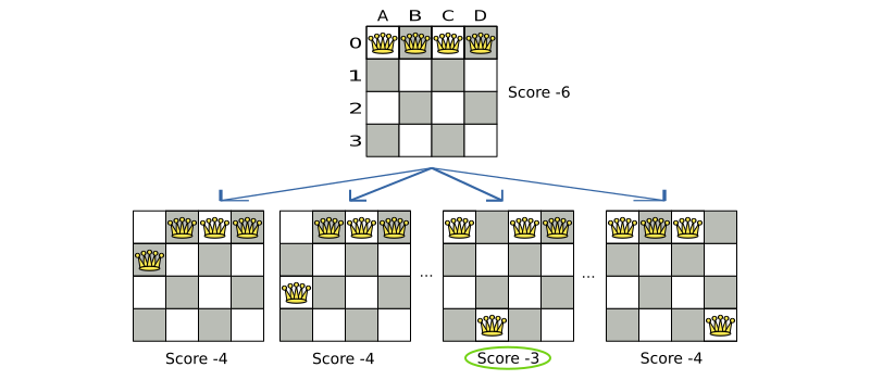
Because the move B0 to B3 has the highest score (-3), it is picked as the next step.
If multiple moves have the same highest score, one is picked randomly, in this case B0 to B3.
Note that C0 to C3 (not shown) could also have been picked because it also has the score -3.
The step is applied on the solution. From that new solution, Local Search tries every move again, to decide the next step after that. It continually does this in a loop, and we get something like this:
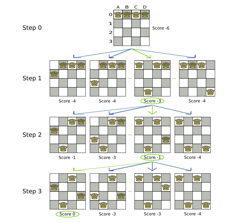
Notice that Local Search doesn’t use a search tree, but a search path. The search path is highlighted by the green arrows. At each step it tries all selected moves, but unless it’s the step, it doesn’t investigate that solution further. This is one of the reasons why Local Search is very scalable.
Local Search solves the four queens problem by starting with the starting solution and make the following steps sequentially:
-
B0 to B3
-
D0 to D2
-
A0 to A1
A naive Local Search configuration solves the four queens problem in three steps, by evaluating only 37 possible solutions (three steps with 12 moves each + one starting solution), which is only a fraction of all 256 possible solutions. It solves 16 queens in 31 steps, by evaluating only 7441 out of 18446744073709551616 possible solutions. By using a Construction Heuristics phase first, it’s even a lot more efficient.
6.2.2. Decide the next step
Local Search decides the next step with the aid of three configurable components:
-
A
MoveSelectorwhich selects the possible moves of the current solution. See move and neighborhood selection. -
An
Acceptorwhich filters out unacceptable moves. -
A
Foragerwhich gathers accepted moves and picks the next step from them.
The solver phase configuration looks like this:
  <localSearch>
    <unionMoveSelector>
      ...
    </unionMoveSelector>
    <acceptor>
      ...
    </acceptor>
    <forager>
      ...
    </forager>
  </localSearch>
In the example below, the MoveSelector generated the moves shown with the blue lines,
the Acceptor accepted all of them and the Forager picked the move B0 to B3.
Turn on trace logging to show the decision making in the log.
Because the last solution can degrade (such as in Tabu Search),
the Solver remembers the best solution it has encountered through the entire search path.
Each time the current solution is better than the last best solution,
the current solution is cloned
and referenced as the new best solution.
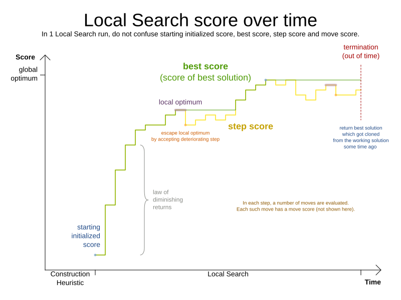
6.2.3. Acceptor
Use an Acceptor (together with a Forager) to activate Tabu Search, Simulated Annealing, Late Acceptance, … For each move it checks whether it is accepted or not.
By changing a few lines of configuration, you can easily switch from Tabu Search to Simulated Annealing or Late Acceptance and back.
You can implement your own Acceptor, but the built-in acceptors should suffice for most needs.
You can also combine multiple acceptors.
6.2.4. Forager
A Forager gathers all accepted moves and picks the move which is the next step.
Normally it picks the accepted move with the highest score.
If several accepted moves have the highest score, one is picked randomly to break the tie.
Breaking ties randomly leads to better results.
|
It is possible to disable breaking ties randomly by explicitly setting
|
Accepted count limit
When there are many possible moves, it becomes inefficient to evaluate all of them at every step. To evaluate only a random subset of all the moves, use:
-
An
acceptedCountLimitinteger, which specifies how many accepted moves should be evaluated during each step. By default, all accepted moves are evaluated at every step.<forager> <acceptedCountLimit>1000</acceptedCountLimit> </forager>
Unlike the N-queens problem, real world problems require the use of acceptedCountLimit.
Start from an acceptedCountLimit that takes a step in less than two seconds.
Turn on INFO logging to see the step times.
Use the Benchmarker to tweak the value.
|
With a low |
Pick early type
A forager can pick a move early during a step, ignoring subsequent selected moves. There are three pick early types for Local Search:
-
NEVER: A move is never picked early: all accepted moves are evaluated that the selection allows. This is the default.<forager> <pickEarlyType>NEVER</pickEarlyType> </forager> -
FIRST_BEST_SCORE_IMPROVING: Pick the first accepted move that improves the best score. If none improve the best score, it behaves exactly like the pickEarlyType NEVER.<forager> <pickEarlyType>FIRST_BEST_SCORE_IMPROVING</pickEarlyType> </forager> -
FIRST_LAST_STEP_SCORE_IMPROVING: Pick the first accepted move that improves the last step score. If none improve the last step score, it behaves exactly like the pickEarlyType NEVER.<forager> <pickEarlyType>FIRST_LAST_STEP_SCORE_IMPROVING</pickEarlyType> </forager>
6.3. Hill climbing (simple local search)
6.3.1. Algorithm description
Hill Climbing tries all selected moves and then takes the best move, which is the move which leads to the solution with the highest score. That best move is called the step move. From that new solution, it again tries all selected moves and takes the best move and continues like that iteratively. If multiple selected moves tie for the best move, one of them is randomly chosen as the best move.
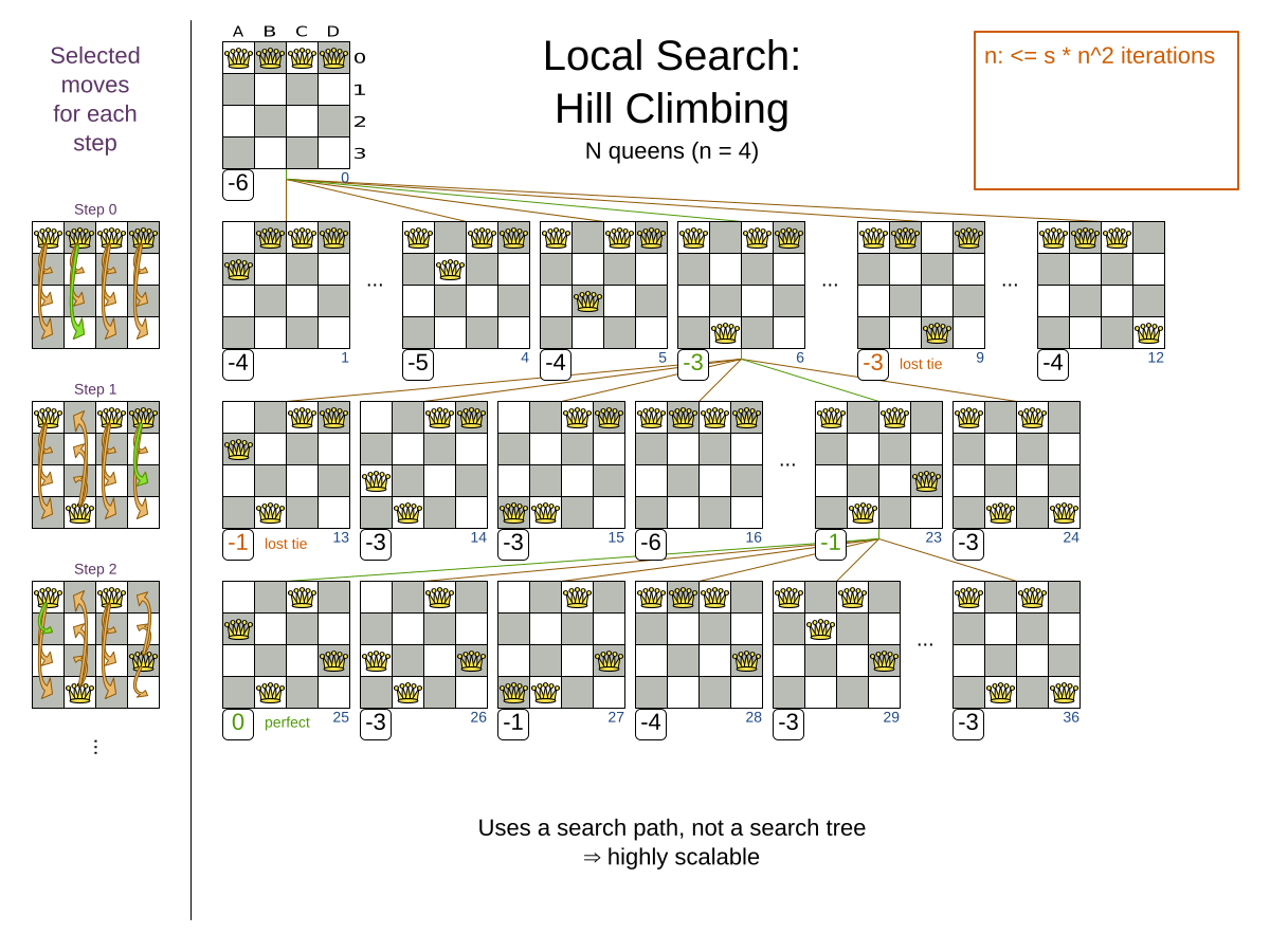
Notice that once a queen has moved, it can be moved again later. This is a good thing, because in an NP-complete problem it’s impossible to predict what will be the optimal final value for a planning variable.
6.3.2. Stuck in local optima
Hill climbing always takes improving moves. This may seem like a good thing, but it’s not: Hill Climbing can easily get stuck in a local optimum. This happens when it reaches a solution for which all the moves deteriorate the score. Even if it picks one of those moves, the next step might go back to the original solution and which case chasing its own tail:
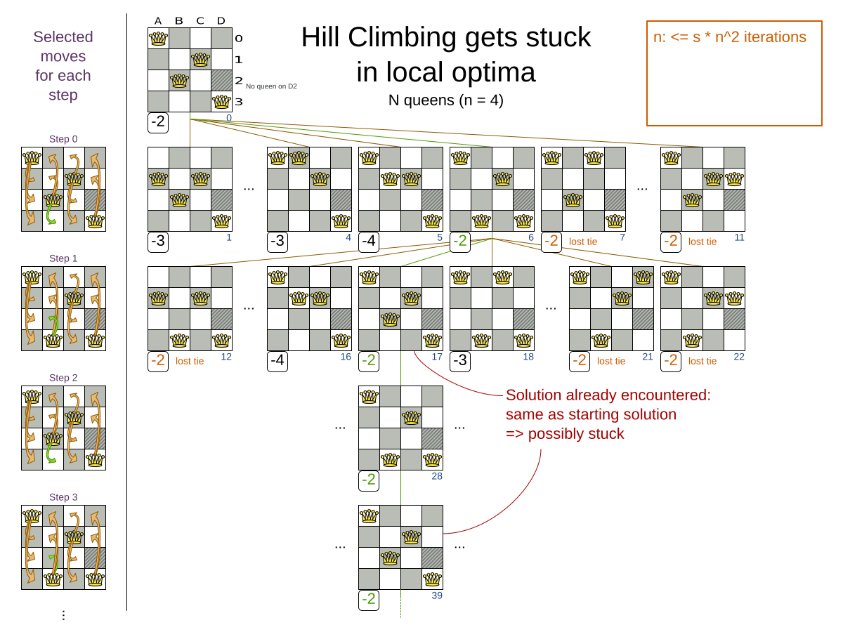
Improvements upon Hill Climbing (such as Tabu Search, Simulated Annealing and Late Acceptance) address the problem of being stuck in local optima. Therefore, it’s recommended to never use Hill Climbing, unless you’re absolutely sure there are no local optima in your planning problem.
6.3.3. Configuration
Simplest configuration:
<localSearch>
<localSearchType>HILL_CLIMBING</localSearchType>
</localSearch>Advanced configuration:
<localSearch>
...
<acceptor>
<acceptorType>HILL_CLIMBING</acceptorType>
</acceptor>
<forager>
<acceptedCountLimit>1</acceptedCountLimit>
</forager>
</localSearch>6.4. Tabu search
6.4.1. Algorithm description
Tabu Search is a Local Search that maintains a tabu list to avoid getting stuck in local optima. The tabu list holds recently used objects that are taboo to use for now. Moves that involve an object in the tabu list, are not accepted. The tabu list objects can be anything related to the move, such as the planning entity, planning value, move, solution, …
See example with entity tabu for four queens, so the queens are put in the tabu list:
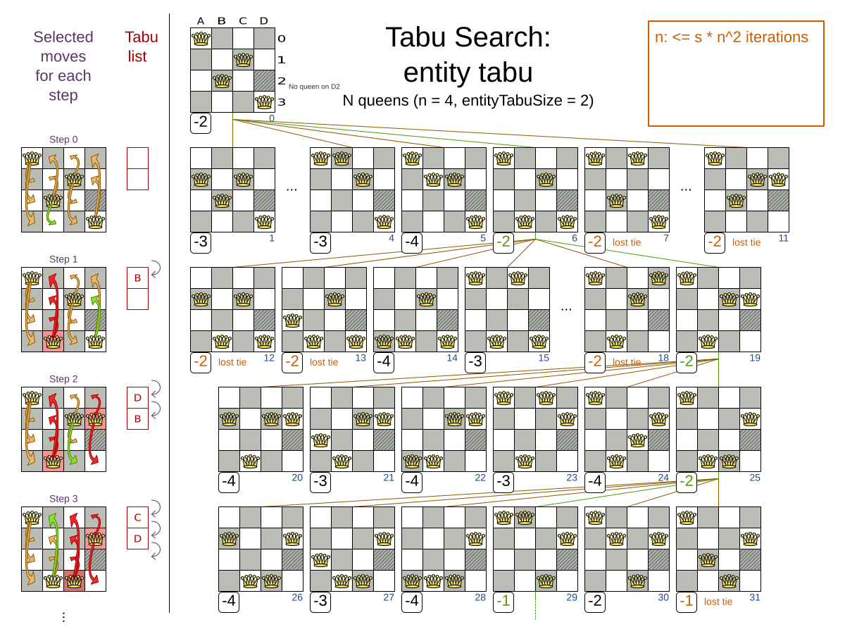
6.4.2. Configuration
Simplest configuration:
<localSearch>
<localSearchType>TABU_SEARCH</localSearchType>
</localSearch>When Tabu Search takes steps it creates one or more tabus. For a number of steps, it does not accept a move if that move breaks tabu. That number of steps is the tabu size. Advanced configuration:
<localSearch>
...
<acceptor>
<entityTabuSize>7</entityTabuSize>
</acceptor>
  <forager>
    <acceptedCountLimit>1000</acceptedCountLimit>
  </forager>
</localSearch>|
A Tabu Search acceptor should be combined with a high |
Timefold Solver implements several tabu types:
-
Planning entity tabu (recommended) makes the planning entities of recent steps tabu. For example, for school timetabling it makes the recently moved lessons tabu. It’s recommended to start with this tabu type.
<acceptor> <entityTabuSize>7</entityTabuSize> </acceptor>To avoid hard coding the tabu size, configure a tabu ratio, relative to the number of entities, for example 2%:
<acceptor> <entityTabuRatio>0.02</entityTabuRatio> </acceptor> -
Planning value tabu makes the planning values of recent steps tabu. For example, for school timetablig it makes the recently assigned timeslots tabu.
<acceptor> <valueTabuSize>7</valueTabuSize> </acceptor>To avoid hard coding the tabu size, configure a tabu ratio, relative to the number of values, for example 2%:
<acceptor> <valueTabuRatio>0.02</valueTabuRatio> </acceptor> -
Move tabu makes recent steps tabu. It does not accept a move equal to one of those steps.
<acceptor> <moveTabuSize>7</moveTabuSize> </acceptor> -
Undo move tabu makes the undo move of recent steps tabu.
<acceptor> <undoMoveTabuSize>7</undoMoveTabuSize> </acceptor>
|
When using move tabu and undo move tabu with custom moves,
make sure that the planning entities do not include planning variables in their |
Sometimes it’s useful to combine tabu types:
<acceptor>
<entityTabuSize>7</entityTabuSize>
<valueTabuSize>3</valueTabuSize>
</acceptor>If the tabu size is too small, the solver can still get stuck in a local optimum. On the other hand, if the tabu size is too large, the solver can be inefficient by bouncing off the walls. Use the Benchmarker to fine tweak your configuration.
6.5. Simulated annealing
6.5.1. Algorithm description
Simulated Annealing evaluates only a few moves per step, so it steps quickly. In the classic implementation, the first accepted move is the winning step. A move is accepted if it doesn’t decrease the score or - in case it does decrease the score - it passes a random check. The chance that a decreasing move passes the random check decreases relative to the size of the score decrement and the time the phase has been running (which is represented as the temperature).
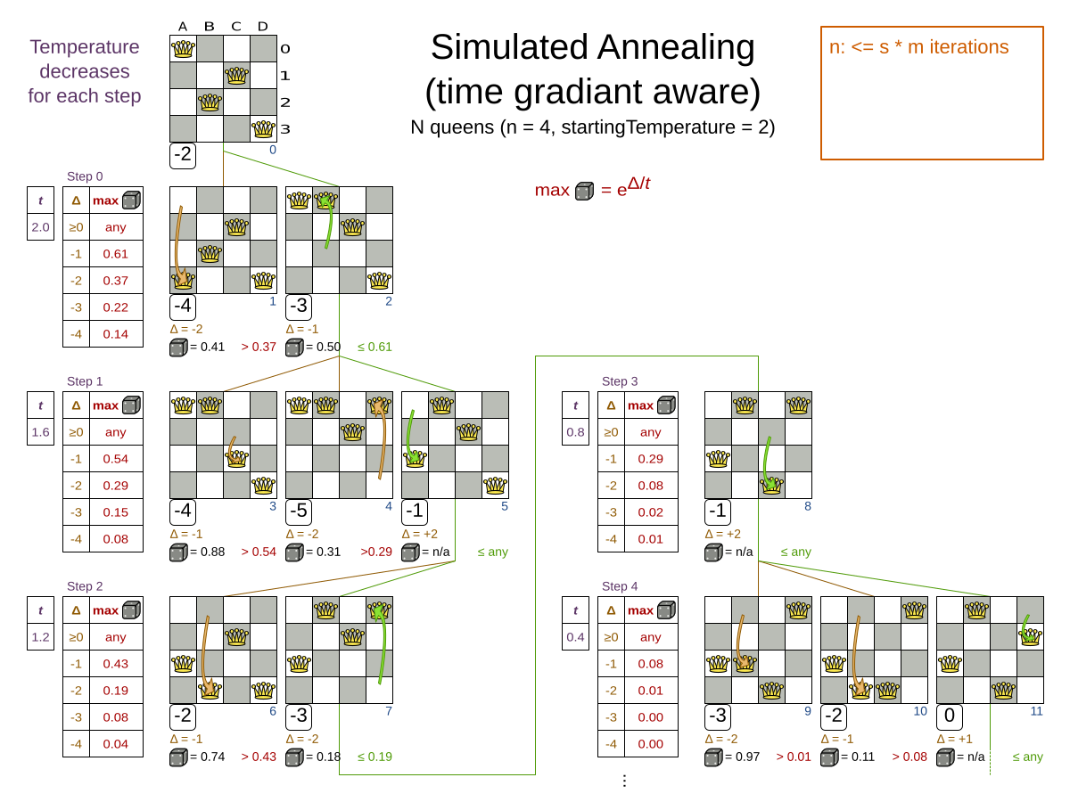
Simulated Annealing does not always pick the move with the highest score, neither does it evaluate many moves per step.
At least at first.
Instead, it gives non improving moves also a chance to be picked, depending on its score and the time gradient of the Termination.
In the end, it gradually turns into Hill Climbing, only accepting improving moves.
6.5.2. Configuration
Start with a simulatedAnnealingStartingTemperature set to the maximum score delta a single move can cause.
Use the Benchmarker to tweak the value.
Advanced configuration:
<localSearch>
...
<acceptor>
<simulatedAnnealingStartingTemperature>2hard/100soft</simulatedAnnealingStartingTemperature>
</acceptor>
<forager>
<acceptedCountLimit>1</acceptedCountLimit>
</forager>
</localSearch>Simulated Annealing should use a low acceptedCountLimit.
The classic algorithm uses an acceptedCountLimit of 1, but often 4 performs better.
Simulated Annealing can be combined with a tabu acceptor at the same time. That gives Simulated Annealing salted with a bit of Tabu. Use a lower tabu size than in a pure Tabu Search configuration.
<localSearch>
...
<acceptor>
<entityTabuSize>5</entityTabuSize>
<simulatedAnnealingStartingTemperature>2hard/100soft</simulatedAnnealingStartingTemperature>
</acceptor>
<forager>
<acceptedCountLimit>1</acceptedCountLimit>
</forager>
</localSearch>6.6. Late acceptance
6.6.1. Algorithm description
Late Acceptance (also known as Late Acceptance Hill Climbing) also evaluates only a few moves per step. A move is accepted if it does not decrease the score, or if it leads to a score that is at least the late score (which is the winning score of a fixed number of steps ago).
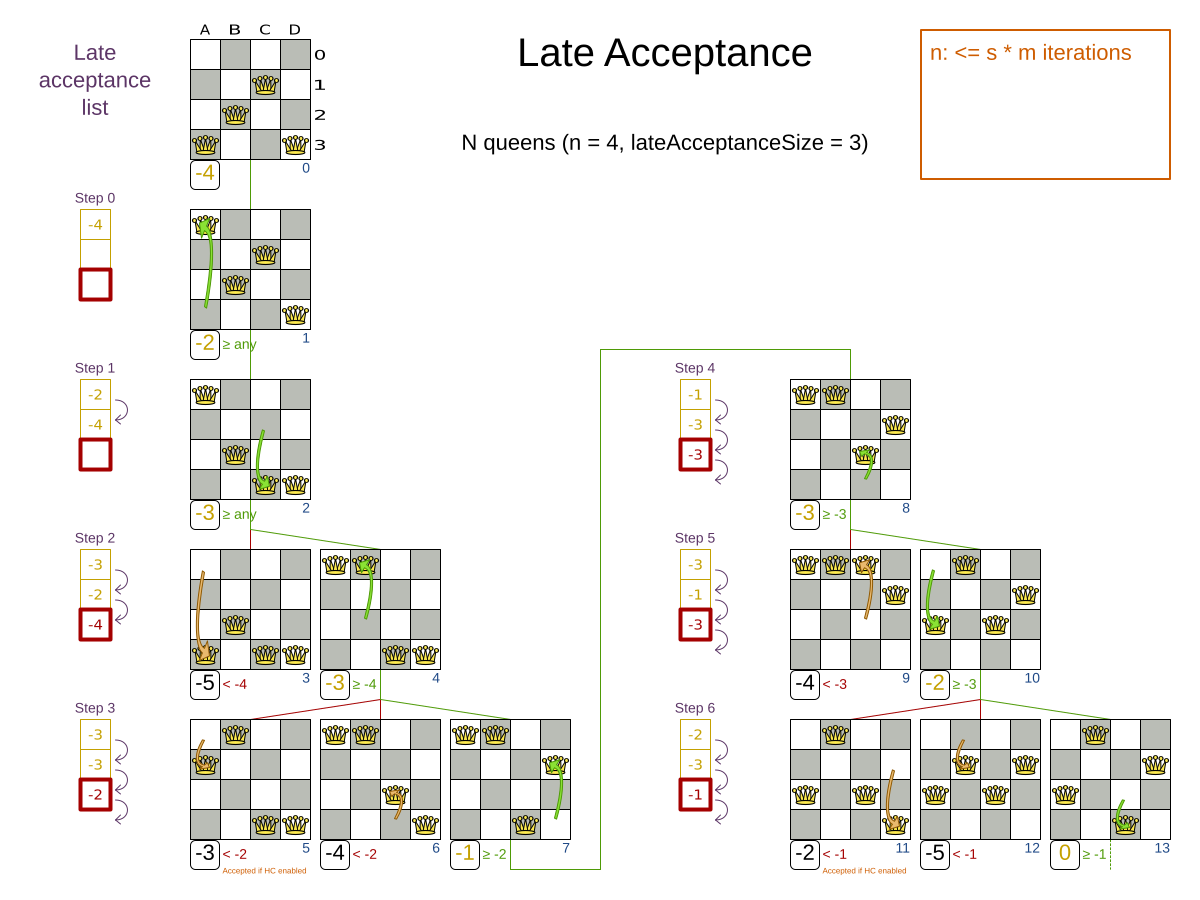
6.6.2. Configuration
Simplest configuration:
<localSearch>
<localSearchType>LATE_ACCEPTANCE</localSearchType>
</localSearch>Late Acceptance accepts any move that has a score which is higher than the best score of a number of steps ago.
That number of steps is the lateAcceptanceSize.
Advanced configuration:
<localSearch>
...
<acceptor>
<lateAcceptanceSize>400</lateAcceptanceSize>
</acceptor>
<forager>
<acceptedCountLimit>1</acceptedCountLimit>
</forager>
</localSearch>Late Acceptance should use a low acceptedCountLimit.
Late Acceptance can be combined with a tabu acceptor at the same time. That gives Late Acceptance salted with a bit of Tabu. Use a lower tabu size than in a pure Tabu Search configuration.
<localSearch>
...
<acceptor>
<entityTabuSize>5</entityTabuSize>
<lateAcceptanceSize>400</lateAcceptanceSize>
</acceptor>
<forager>
<acceptedCountLimit>1</acceptedCountLimit>
</forager>
</localSearch>6.7. Great Deluge
6.7.1. Algorithm description
Great Deluge algorithm is similar to the Simulated Annealing algorithm, it evaluates only a few moves per steps, so it steps quickly. The first accepted move is the winning step. A move is accepted only if it is not lower than the score value (water level) that we are working with. It means Great Deluge is deterministic and opposite of Simulated Annealing has no randomization in it. The water level is increased after every step either about the fixed value or by percentual value. A gradual increase in water level gives Great Deluge more time to escape from local maxima.
6.7.2. Configuration
Simplest configuration:
<localSearch>
<localSearchType>GREAT_DELUGE</localSearchType>
</localSearch>Great Deluge takes as starting water level best score from construction heuristic and uses default rain speed ratio. Advanced configuration:
<localSearch>
...
<acceptor>
<greatDelugeWaterLevelIncrementRatio>0.00000005</greatDelugeWaterLevelIncrementRatio>
</acceptor>
<forager>
<acceptedCountLimit>1</acceptedCountLimit>
</forager>
</localSearch>Timefold Solver implements two water level increment options:
If greatDelugeWaterLevelIncrementScore is set, the water level is increased by a constant value.
<acceptor>
<greatDelugeWaterLevelIncrementScore>10</greatDelugeWaterLevelIncrementScore>
</acceptor>To avoid hard coding the water level increment, configure a greatDelugeWaterLevelIncrementRatio (recommended) when the water level is increased by percentual value, so there is no need to know the size of the problem or value of a scoring function.
<acceptor>
<greatDelugeWaterLevelIncrementRatio>0.00000005</greatDelugeWaterLevelIncrementRatio>
</acceptor>The algorithm takes as starting value the best score from the construction heuristic. Use the Benchmarker to fine-tune tweak your configuration.
6.8. Step counting hill climbing
6.8.1. Algorithm description
Step Counting Hill Climbing also evaluates only a few moves per step. For a number of steps, it keeps the step score as a threshold. A move is accepted if it does not decrease the score, or if it leads to a score that is at least the threshold score.
6.8.2. Configuration
Step Counting Hill Climbing accepts any move that has a score which is higher than a threshold score.
Every number of steps (specified by stepCountingHillClimbingSize), the threshold score is set to the step score.
<localSearch>
...
<acceptor>
<stepCountingHillClimbingSize>400</stepCountingHillClimbingSize>
</acceptor>
<forager>
<acceptedCountLimit>1</acceptedCountLimit>
</forager>
</localSearch>Step Counting Hill Climbing should use a low acceptedCountLimit.
Step Counting Hill Climbing can be combined with a tabu acceptor at the same time, similar as shown in the Late Acceptance section.
6.9. Strategic oscillation
6.9.1. Algorithm description
Strategic Oscillation is an add-on, which works especially well with Tabu Search. Instead of picking the accepted move with the highest score, it employs a different mechanism: If there’s an improving move, it picks it. If there’s no improving move however, it prefers moves which improve a softer score level, over moves which break a harder score level less.
6.9.2. Configuration
Configure a finalistPodiumType, such as in a Tabu Search configuration:
<localSearch>
...
<acceptor>
<entityTabuSize>7</entityTabuSize>
</acceptor>
<forager>
<acceptedCountLimit>1000</acceptedCountLimit>
<finalistPodiumType>STRATEGIC_OSCILLATION</finalistPodiumType>
</forager>
</localSearch>The following finalistPodiumTypes are supported:
-
HIGHEST_SCORE(default): Pick the accepted move with the highest score. -
STRATEGIC_OSCILLATION: Alias for the default strategic oscillation variant. -
STRATEGIC_OSCILLATION_BY_LEVEL: If there is an accepted improving move, pick it. If no such move exists, prefer an accepted move which improves a softer score level over one that doesn’t (even if it has a better harder score level). A move is improving if it’s better than the last completed step score. -
STRATEGIC_OSCILLATION_BY_LEVEL_ON_BEST_SCORE: LikeSTRATEGIC_OSCILLATION_BY_LEVEL, but define improving as better than the best score (instead of the last completed step score).
6.10. Variable neighborhood descent
6.10.1. Algorithm description
Variable Neighborhood Descent iteratively tries multiple move selectors in original order (depleting each selector entirely before trying the next one), picking the first improving move (which also resets the iterator back to the first move selector).
|
Despite that VND has a name that ends with descent (from the research papers), the implementation will ascend to a higher score (which is a better score). |
6.10.2. Configuration
Simplest configuration:
<localSearch>
<localSearchType>VARIABLE_NEIGHBORHOOD_DESCENT</localSearchType>
</localSearch>Advanced configuration:
<localSearch>
<unionMoveSelector>
<selectionOrder>ORIGINAL</selectionOrder>
<changeMoveSelector/>
<swapMoveSelector/>
...
</unionMoveSelector>
<acceptor>
<acceptorType>HILL_CLIMBING</acceptorType>
</acceptor>
    <forager>
      <pickEarlyType>FIRST_LAST_STEP_SCORE_IMPROVING</pickEarlyType>
    </forager>
</localSearch>Variable Neighborhood Descent doesn’t scale well, but it is useful in some use cases with a very erratic score landscape.
7. Multi-threaded solving
|
Multi-threaded solving is a commercial feature of Timefold Solver Enterprise Edition. It is not open source, and it is free for development use only. Learn more about Timefold. |
Read about multi-threaded solving in the Multi-threaded solving section of the Enterprise Edition manual.