Designing the Timefold logo

Every new company needs a logo. So does Timefold. When starting a company, one of the most fun tasks is creating the logo. Far more exciting than VAT accounting, I can tell you.
Of course, a good logo is important: It’s hard to change. It must be able to stand the test of time. It should fit on a variety of media. So we hired a professional to help us: Ivo Blomme, a digital and brand designer with years of experience. He took us through the process of creating a good logo. Based on our input, he created these:
The left one is based on the rectangles of a physical calendar. The right one, with a fold in it, is based on a fold in space and time. Which logo would you have picked?
It was a though call, but we ended going for the second one. It’s loosely based on the idea of folding space and time:

Our designer even showed us how it would look on digital devices:
Now, we don’t have any plans to create a mobile app. But it would look good, wouldn’t it?

Same coffee, same shoes, same plan: the beauty of no surprises
Same coffee, same shoes, same plan
I am, by most reasonable definitions, a creature of habit.
Same coffee every morning. Same brand of shoes for years (and a small grieving period whenever a pair finally gives up and I have to go shopping for new ones). Same route to the office. Same seat at the dinner table. My partner finds this both endearing and, occasionally, a little bit boring.
Now, this is not because I hate change. I genuinely enjoy exploring new things. New countries, new conferences, new restaurants, new problems to model. But underneath all that exploring, there is a quiet preference humming away: I like knowing what I’m going to get.
It probably won’t surprise you that this same preference is what nudged me toward software engineering in the first place. There’s something deeply satisfying about a function. You put 2 and 3 in, you get 5 out. You run it again tomorrow on a different machine, in a different timezone, after a different coffee, and you still get 5.
Most of my career has been built on that simple promise: given the same inputs, give me the same outputs. It’s how you debug things. It’s how you trust things. It’s how you sleep at night when your code is running in production.
So when I tell people I now work at an AI company, I sometimes get a raised eyebrow. The implied question is usually:
“Wait. You? The guy who reorders the exact same dish every time? Working in AI?”
I guess that’s fair…
The thing most people now call “AI”
When most people hear “AI” in 2026, their brain jumps straight to Generative AI. ChatGPT. Image generators. Coding assistants. The kind of AI that, by design, can give you a slightly different answer every time you ask. Sometimes wildly different.
That non-determinism is actually a feature for Gen AI. If you ask for “a haiku about suffering through allergies”, you don’t want the exact same poem every time. You want variety, creativity, surprise.

But not everything runs on poems. A lot of the world runs on plans. Plans for delivery routes. Plans for shift rosters. Plans for which truck picks up which order at which time. And for those, “a slightly different answer every time” is not charming. It’s a nightmare.
Being predictable isn’t boring, it’s a superpower
Here’s what I love about working at Timefold: our solver is AI, but it’s deterministic. Same data in, same CPU budget, same answer comes out.
That sentence sounds unremarkable until you’ve spent a few years debugging planning systems where it wasn’t true. Where re-running the same input gave you a different roster, a different route plan, a different recommendation… and you had no way to tell whether the difference came from the algorithm doing its job, from a bug, or from cosmic radiation (this is not sci-fi… it happens and is one of the main reasons why building data centers in space is hard).
Determinism unlocks a bunch of things that are otherwise really hard:
- You can reproduce bugs. A planner reports a weird shift assignment? You re-run the same dataset and you get the exact same weird assignment. Now you can actually investigate it.
- You can test. Real tests, with real assertions, that don’t randomly fail every third CI run. Your tests don’t say “the solution should be roughly this.” They say “the solution is this.”
- You can A/B compare changes. Want to know if your new constraint tweak actually improved things? Run before and after on the same data. Any difference you see is caused by your change, not by the dice.
- You can build trust. Planners using the system see the same plan twice and start to believe in it. Show them a different answer each time and you’re toast, no matter how good the math is.
This isn’t a small thing. It’s the difference between a system you can operate and a system you have to babysit.
Determinism is the old next thing!
I get why determinism doesn’t make for exciting marketing copy. “Our AI gives you the same answer every time” is not going to trend on LinkedIn. It sounds almost like a downgrade in an era where people expect their AI to dazzle them with novelty.

But for planning problems, where decisions affect real shifts, real deliveries, real people, boring is exactly what you want. You want a system that behaves the same way on a Tuesday as it does on a Friday. You want a result you can defend, reproduce, and test.
In other words, you want your planning AI to be a bit of a creature of habit. Same input, same output. Same coffee, same shoes.
Honestly? It’s my favorite kind of magic. 🙂

Timefold Raises $13M as AI Drives Demand for Routing and Scheduling APIs
- Led by Alstin Capital, co-investor Kompas VC, and continued backing from Lakestar and Smartfin
- ARR grew 4x in 2025 as enterprises like NEC Software Solutions, CBRE, Lufthansa, Thales, and Subaru embedded Timefold's APIs into mission-critical scheduling solutions
- Funding will accelerate US expansion and platform product development
%201.avif)
GENT, BELGIUM - 23 June 2026 - Timefold, the developer platform for vehicle routing and shift scheduling APIs, today announced the close of a $13M Series A funding round led by Alstin Capital, with co-investor Kompas VC, and continued backing from existing investors Lakestar and Smartfin.
Timefold enables software teams in field service and workforce management to easily integrate enterprise-grade scheduling optimization into the solutions they are supporting.
The round follows a year of commercial momentum. In 2025, Timefold grew its annual recurring revenue 4x, driven by enterprises and software vendors embedding its APIs into mission-critical field service operations and scheduling workflows.
The new funding will accelerate Timefold’s US expansion and support the growing enterprise demand for easy-to-integrate scheduling optimization infrastructure.
"Schedules run the world," says Maarten Vandenbroucke, CEO of Timefold. "We are all at the mercy of a schedule, and so are the millions of frontline workers whose days depend on getting it right. As software becomes increasingly autonomous, optimization becomes foundational infrastructure. That’s why we believe Timefold is the best vehicle routing scheduler. Our platform gives software builders the ability to embed enterprise-grade decision intelligence into their applications, enabling better outcomes for businesses, workers, and customers alike."
Scheduling optimization for the AI builder era
The rise of AI agents is creating a new generation of software that can understand requests and generate schedules. But LLM-generated schedules don't always work in production because of its probabilistic nature.
Timefold offers AI-powered software powered by a deterministic algorithm to tackle large-scale scheduling challenges. It enables teams to automate decisions on which technician should visit which customer, how to respond when a technician calls in sick, or how to create a shift schedule that is fair, compliant, and fully staffed.
That decision-making is particularly essential in field service, where operations are among the hardest scheduling environments to manage. Every day, companies must coordinate thousands of jobs while balancing technician qualifications, SLAs, labor regulations, travel times, customer availability, and last-minute disruptions in real time.
Freeing the world from wasteful scheduling
Handling any constraint, any scale, and any level of operational complexity, Timefold delivers measurable results. A global real estate services company reduced drive time by up to 33%, cut distance traveled by 43%, and eliminated overtime entirely using Timefold’s Field Service Routing solution. A major US retail staffing provider reduced a scheduling process that previously took 10 weeks to just 10 minutes using Timefold’s Employee Shift Scheduling model.
Enterprise customers, including NEC Software Solutions (NECSWS), CBRE, Orange Telecom, ADP, and Lufthansa, rely on Timefold to power operational scheduling workflows where inefficiency directly impacts profitability, customer experience, and workforce productivity.
“We chose Timefold because it gave us a practical way to bring advanced planning AI into real operations without slowing down delivery,” says Kay Aston of NECSWS. “Their technology helped us move faster, create clear operational value, and strengthen how we bring optimization capabilities to our customer base.”
Scheduling as a foundational component
Timefold believes scheduling optimization will become a foundational component of software in the AI era. As software development becomes more accessible and AI-generated applications become commonplace, the company’s vision is to become the default platform for building, deploying, and operating scheduling optimization models, enabling any software team to solve complex scheduling problems at scale.
"What matters in mission-critical scheduling isn't creativity, it's correctness: a shift roster or a vehicle route has to be right, compliant, and reproducible every time. LLMs aren't built for that. What convinced us to lead Timefold's round was the team's understanding of exactly that constraint, and what they've built around it. They've taken a battle-tested open source optimization engine and wrapped it in modular products that any enterprise can deploy, without needing a team of mathematicians. That's how deep optimization technology becomes infrastructure, and we believe Timefold is best placed to own that category”, says Alexander Meyer-Scharenberg, Partner at Alstin Capital.

How upskilling technicians unlocks field service routing efficiency
In telecom, utilities, and HVAC, not every technician can handle every job. A field engineer certified for fiber installations may or may not also hold IP networking qualifications. These skill gaps seem like a workforce planning issue, but they compound into a routing problem that costs companies millions in unnecessary travel time and lost capacity.
The question worth asking: how much money are you leaving on the table? We've modeled it across multiple scenarios and quantified the answer in dollars.
The problem
Consider a simplified but representative example: 5 service visits, 2 technicians, each visit requiring one specific skill, each technician holding one skill.
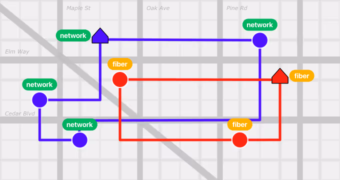
The routing algorithm has no choice but to send both technicians across the city to match skills to jobs, even when a geographically closer technician could handle the work with a single additional qualification.
The result is excessive travel time, reduced daily capacity, and lower customer face time.
The opportunity
Now consider what changes when one technician is cross-trained.
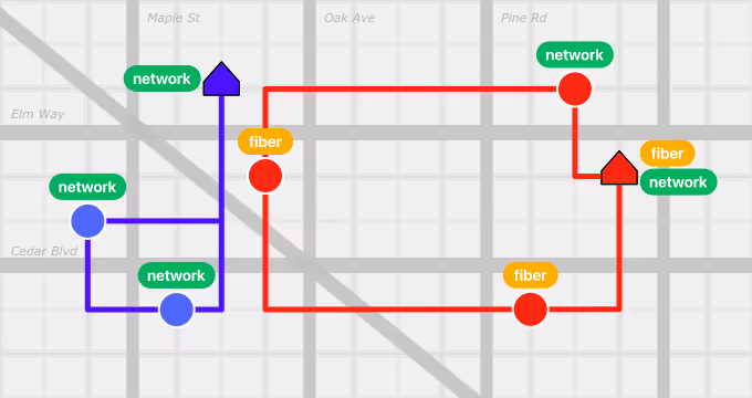
With the red technician qualified for network jobs as well, the routing engine can assign jobs more efficiently, and the other technician's route contracts immediately.
Extend that to both technicians holding all relevant skills, and both routes shorten substantially.

Total travel time drops significantly, freeing capacity for additional visits or higher-quality customer interactions. The productivity gain is real and measurable, not theoretical.
The benchmarks
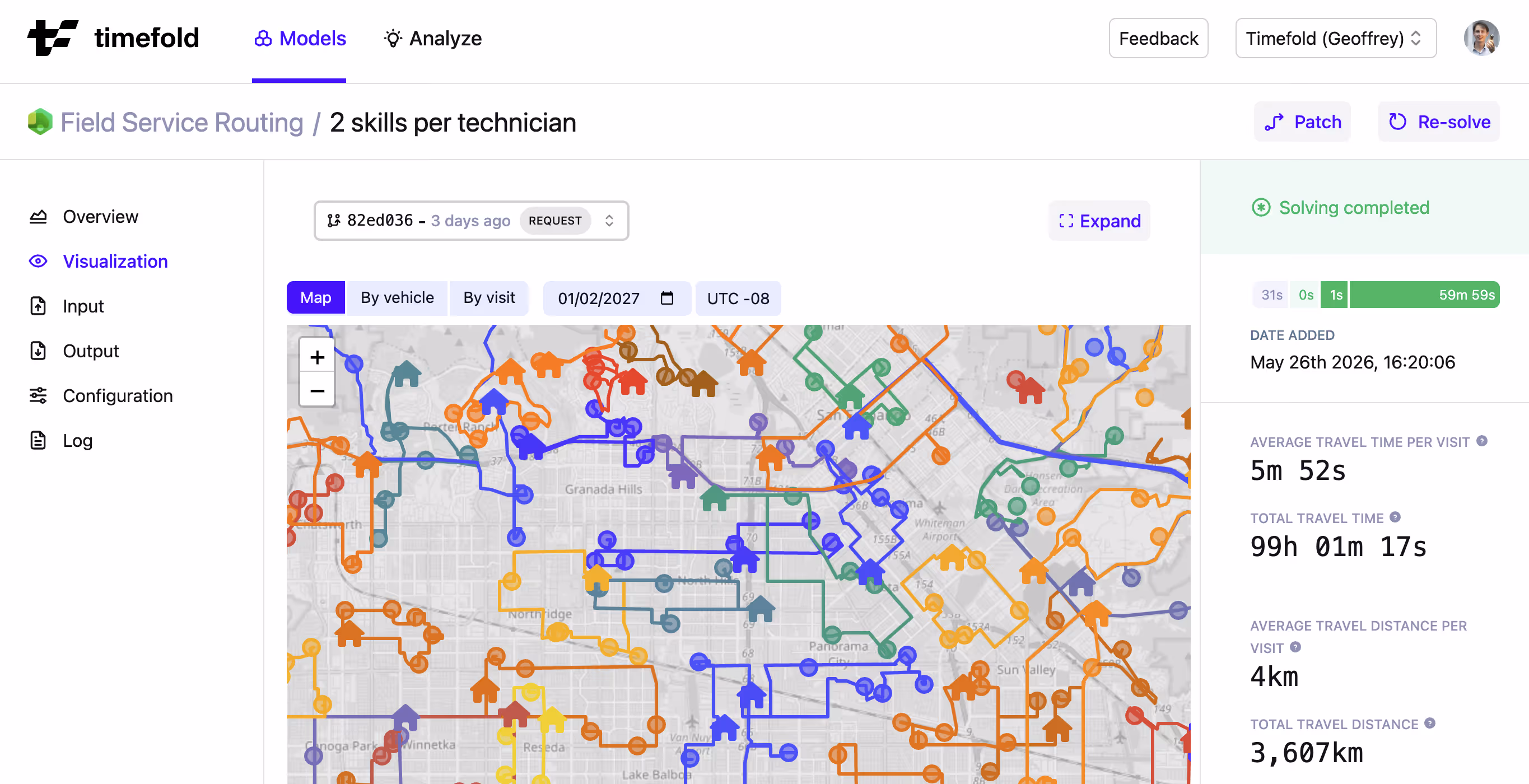
To move beyond simplified examples, we modeled this against a Los Angeles dataset with 1,012 service visits, 253 technicians, and three distinct skill types. Each job requires exactly one skill, but coverage of technician skills varies.
We ran three scenarios to simulate progressive upskilling investment:
- 1 skill per technician (baseline): No cross-training. Each technician holds exactly one qualification.
- 2 skills per technician: Every technician is trained on one additional skill.
- 3 skills per technician: Full cross-training. Every technician holds all three qualifications.
All three scenarios were solved using our Field Service Routing API.
The results
The productivity gains from upskilling are significant and consistent.
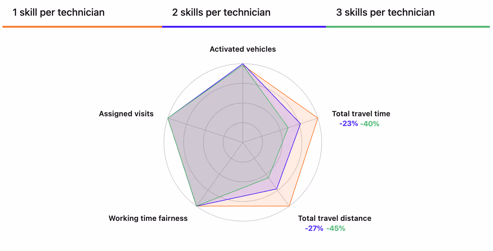
Moving from 1 to 2 skills per technician reduces travel time by 23%. For a technician averaging 2 hours of daily drive time, that's over 26 minutes saved per day, which compounds to 88 hours per year at 200 working days. At a $50/hour wage rate, that amounts to $4,400 in recovered productivity per technician annually.
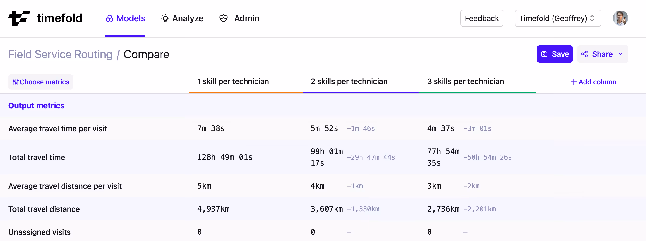
Moving from 2 to 3 skills reduces travel time by a further 17%, adding another $3,400 per technician per year.
Partial upskilling
Partial upskilling still delivers meaningful ROI. Training only half the workforce on a second skill still yields a 14% reduction in travel time: $2,800 per technician per year across the organization.
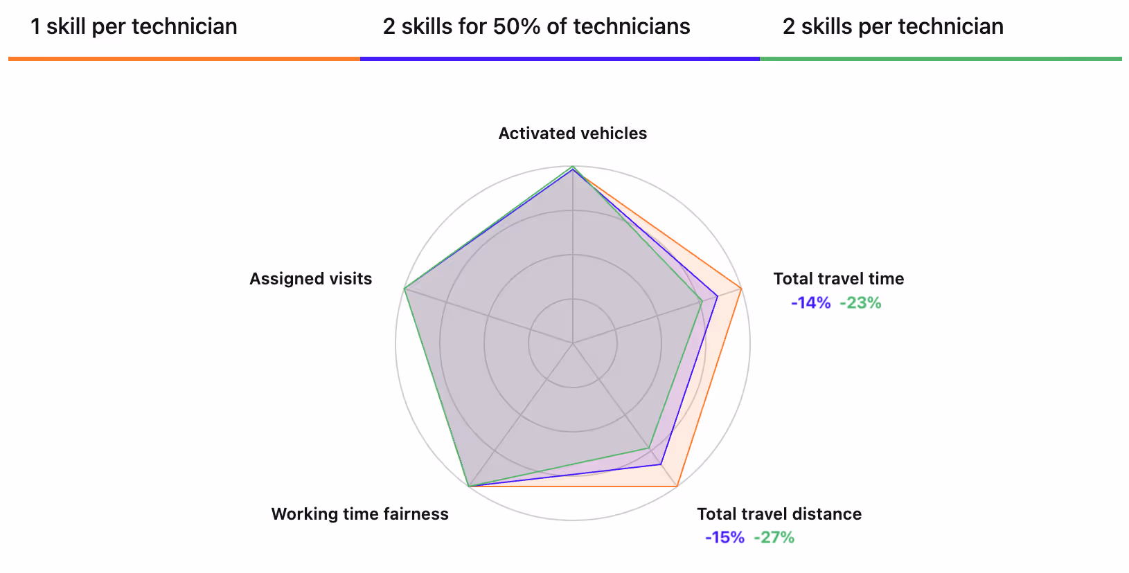
Interestingly, the ROI in this scenario reaches $5,600 per trained technician annually, as the routing engine concentrates efficiency gains through the newly cross-trained subset. The aggregate company-wide return is lower, but the per-investment return is higher; a useful lever for phased rollout decisions.
Conclusion
This analysis is based on a single dataset from a single metropolitan region. Field operations at an enterprise scale are considerably more complex, involving non-uniform skill distributions, varying geographic densities, and routing challenges across hundreds of service regions and time periods.
This study demonstrates the structure of the ROI opportunity. The specific numbers will vary with your workforce composition and operational footprint, but the finding is consistent with what we observe across our customer base.
The most accurate projections come from running these simulations against your own data. We can do exactly that and give you a defensible, operations-specific estimate of the value of upskilling investments before you make them.

How much fuel can route optimization actually save?
Fuel costs are rarely the largest expense on a field service balance sheet, but they are often the most visible indicator of operational waste. For most fleet managers, the primary challenge is not deciding whether to optimize. The real challenge is determining exactly how much margin is being lost to the road and how to capture that value in a way that satisfies a CFO.
That second part matters more than vendors usually admit. After deploying optimization, fleets often see metrics improve in some places and degrade in others. Before deciding on scheduling optimization, it is worth knowing what the typical savings range looks like, what drives the spread, and how to measure savings in a way that survives a CFO review.
What savings to expect
Across published case studies and operator interviews, field service operations moving from dispatcher-built routes to automated route optimization typically see drive time fall 15% to 30%. Fuel consumption tracks closely, with reported savings of 10% to 25% depending on territory geometry and stop density.
Two things drive the spread:
- Starting point. Fleets coming off paper routes or single-dispatcher Excel tend to land at the high end. Operations already running a basic FSM with simple capacity rules often start at 5% to 10% savings and grow from there as constraints get tuned.
- Constraint stack. A fleet with skill matching, time windows, SLAs, and overtime rules is already hard manage manually. Add multi-vehicle stops, dependent jobs, or rolling time-windows, and it becomes impossible. So, the complexer the operations, the harder it is for the human planner to zoom out, or to think about efficiency. In these cases, a feasible schedule is already a big win, but fuel costs are not something taken into account.
According to Service Council research, the cost to dispatch a technician ranges from $250 in urban environments to as high as $2,500 for rural or multi-day jobs. When you combine this with the US National average fuel price hovering at $4.50 per gallon (May 2nd, 2026),high costs are draining your service profits.
[highlight]
A useful baseline: A 200-technician operation averaging 90 miles per tech per day at 20 mpg burns roughly 900 gallons daily. At the current national average of $4.50 per gallon, that is $4,050 daily, or $1,012,500 per year (based on a 250-day work year).
- A 15% reduction in fuel usage/mileage results in $151,875 in annual savings.
- A 25% reduction results in $253,125 in annual savings.
Overtime savings often add another 30% to 50% on top because fewer hours behind the wheel means fewer late-day SLA scrambles.
[highlight]
How to measure routing optimization savings credibly
Three traps operations leaders fall into:
- Comparing optimized days against manual days that were not comparable. Manual routing tends to do better on light days and worse on heavy days. If the rollout coincides with a seasonal lull, the comparison flatters the optimizer. The fix: index by stops-per-day or jobs-per-tech, not raw miles.
- Counting gross miles, not the right miles. "Miles driven" includes deadhead, on-job movement, and home-to-first-stop legs. Optimization should mostly cut the first two. If you measure all three together, returns look smaller than they are. Pull a week of telematics data and split it before you set the baseline.
- Relying on "Holdout" territories. Comparing one territory against another is often flawed because no two regions have the same density or traffic patterns. The cleanest measurement approach is a parallel plan analysis: run your manual process as usual, but simultaneously feed the exact same job data into the optimizer. Compare the two resulting schedules for the same day to see the true delta in miles and cost.
Where different tools fit in the fuel-cost picture
The market often gets discussed as if every "route optimization" product is the same thing. They are not. Four product categories show up in fuel-reduction conversations, each doing a different job:
The right pick depends on what you already have. If you are running Salesforce Field Service and your dispatch lives there, the question is whether the bundled optimizer is hitting the savings range above. If not, you might need to call out to a scheduling API to fill the gap. If you are running a homegrown ops stack, you need a solution that provides both the distance data and the solver engine to find the best routes.
Three questions to expose if a vendor can deliver
These questions help separate vendors that can actually deliver savings from those that just quote them:
- Can your engine support all our hard constraints simultaneously? If an optimizer cannot handle every real-world rule (skills, windows, SLAs) at the same time, it will produce "invalid" routes. When a planner has to manually fix these, any theoretical fuel savings immediately vanish.
- How can the schedule adapt to real-world events? Most fuel waste happens after disruptions like sick technicians, overrun jobs, or cancellations. If the engine cannot re-solve the schedule in seconds during the day, the efficiency you gained in the morning is lost by lunch.
- How do we prove the savings during a pilot? Avoid "before and after" comparisons. Ask the vendor to perform a "shadow" run where they optimize a historical week of your real data and compare it against the actual routes your team drove.
Fuel cost is the easiest win in field service. The savings are real, the math is settled, and the technology is mature. What is left is fit: with your stack, your constraints, and how your team actually runs.

Three optimizations to make your Timefold Solver faster
Our friends at Dots & Lines recently claimed they made their Timefold Solver 17x faster and they're not wrong. With our IncrementalScoreCalculator, you can absolutely get there. But it comes bundled with months of effort, sacrificed explainability, and constraints that become a nightmare to maintain or extend.
There's a better way. In this post, we'll apply three targeted optimizations to the same course scheduling problem they used and walk away with a 91% speedup while keeping your constraints clean, testable, and easy to change.
The Setup
We're using the code from the Dots & Lines article as our baseline. If you haven't read it, don't worry, we'll cover everything you need here. One difference: we're measuring things slightly differently. We're using the comp06 dataset (where they saw the biggest gains), running for 1 minute with a 15-second JVM warmup, averaging across 10 runs in separate JVM processes, and using -Xmx1g -XX:+UseParallelGC -XX:+UseCompactObjectHeaders to fine-tune performance and keep the noise out. This gives us a more stable baseline than a single long run.
Here's the starting constraint implementation:
public class CurriculumCourseConstraintProvider implements ConstraintProvider {
    @Override
    public Constraint[] defineConstraints(ConstraintFactory factory) {
        return new Constraint[]{
                conflictingLecturesDifferentCourseInSamePeriod(factory),
                conflictingLecturesSameCourseInSamePeriod(factory),
                roomOccupancy(factory),
                unavailablePeriodPenalty(factory),
                roomCapacity(factory),
                minimumWorkingDays(factory),
                curriculumCompactness(factory),
                roomStability(factory)
        };
    }
    // ************************************************************************
    // Hard constraints
    // ************************************************************************
    Constraint conflictingLecturesDifferentCourseInSamePeriod(ConstraintFactory factory) {
        return factory.forEach(CourseConflict.class)
                .join(Lecture.class,
                        equal(CourseConflict::getLeftCourse, Lecture::getCourse))
                .join(Lecture.class,
                        equal((courseConflict, lecture1) -> courseConflict.getRightCourse(), Lecture::getCourse),
                        equal((courseConflict, lecture1) -> lecture1.getPeriod(), Lecture::getPeriod))
                .filter(((courseConflict, lecture1, lecture2) -> lecture1 != lecture2))
                .penalize(ONE_HARD,
                        (courseConflict, lecture1, lecture2) -> courseConflict.getConflictCount())
                .asConstraint("conflictingLecturesDifferentCourseInSamePeriod");
    }
    Constraint conflictingLecturesSameCourseInSamePeriod(ConstraintFactory factory) {
        return factory.forEachUniquePair(Lecture.class,
                        equal(Lecture::getPeriod),
                        equal(Lecture::getCourse))
                .penalize(ONE_HARD,
                        (lecture1, lecture2) -> 1 + lecture1.getCurriculumSet().size())
                .asConstraint("conflictingLecturesSameCourseInSamePeriod");
    }
    Constraint roomOccupancy(ConstraintFactory factory) {
        return factory.forEachUniquePair(Lecture.class,
                        equal(Lecture::getRoom),
                        equal(Lecture::getPeriod))
                .penalize(ONE_HARD)
                .asConstraint("roomOccupancy");
    }
    Constraint unavailablePeriodPenalty(ConstraintFactory factory) {
        return factory.forEach(UnavailablePeriodPenalty.class)
                .join(Lecture.class,
                        equal(UnavailablePeriodPenalty::getCourse, Lecture::getCourse),
                        equal(UnavailablePeriodPenalty::getPeriod, Lecture::getPeriod))
                .penalize(ofHard(10))
                .asConstraint("unavailablePeriodPenalty");
    }
    // ************************************************************************
    // Soft constraints
    // ************************************************************************
    Constraint roomCapacity(ConstraintFactory factory) {
        return factory.forEach(Lecture.class)
                .filter(lecture -> lecture.getStudentSize() > lecture.getRoom().getCapacity())
                .penalize(ofSoft(1),
                        lecture -> lecture.getStudentSize() - lecture.getRoom().getCapacity())
                .asConstraint("roomCapacity");
    }
    Constraint minimumWorkingDays(ConstraintFactory factory) {
        return factory.forEach(Lecture.class)
                .groupBy(Lecture::getCourse, countDistinct(Lecture::getDay))
                .filter((course, dayCount) -> course.getMinWorkingDaySize() > dayCount)
                .penalize(ofSoft(5),
                        (course, dayCount) -> course.getMinWorkingDaySize() - dayCount)
                .asConstraint("minimumWorkingDays");
    }
    Constraint curriculumCompactness(ConstraintFactory factory) {
        return factory.forEach(Curriculum.class)
                .join(Lecture.class,
                        filtering((curriculum, lecture) -> lecture.getCurriculumSet().contains(curriculum)))
                .ifNotExists(Lecture.class,
                        equal((curriculum, lecture) -> lecture.getDay(), Lecture::getDay),
                        equal((curriculum, lecture) -> lecture.getTimeslotIndex(), lecture -> lecture.getTimeslotIndex() + 1),
                        filtering((curriculum, lectureA, lectureB) -> lectureB.getCurriculumSet().contains(curriculum)))
                .ifNotExists(Lecture.class,
                        equal((curriculum, lecture) -> lecture.getDay(), Lecture::getDay),
                        equal((curriculum, lecture) -> lecture.getTimeslotIndex(), lecture -> lecture.getTimeslotIndex() - 1),
                        filtering((curriculum, lectureA, lectureB) -> lectureB.getCurriculumSet().contains(curriculum)))
                .penalize(ofSoft(2))
                .asConstraint("curriculumCompactness");
    }
    Constraint roomStability(ConstraintFactory factory) {
        return factory.forEach(Lecture.class)
                .groupBy(Lecture::getCourse, countDistinct(Lecture::getRoom))
                .filter((course, roomCount) -> roomCount > 1)
                .penalize(HardSoftScore.ONE_SOFT,
                        (course, roomCount) -> roomCount - 1)
                .asConstraint("roomStability");
    }
}
With that out of the way, let's get to the optimizations!
Upgrading to the latest Timefold Solver
The original article used Timefold Solver 1.21.0, a version which is more than a year old at the time of writing this article. Since then, there have been many optimizations and bugfixes to the Timefold Solver codebase, and upgrading to the latest version of Timefold Solver is the first step to get optimal performance.
While upgrading to the newest Timefold Solver version did not significantly impact baseline performance in this use case, the newer versions do come with extra features you can implement to improve performance.
Precomputing static joins
Let's consider the conflictingLecturesDifferentCourseInSamePeriod constraint:
return factory.forEach(CourseConflict.class)
    .join(Lecture.class,
            equal(CourseConflict::getLeftCourse, Lecture::getCourse))
    .join(Lecture.class,
            equal((courseConflict, lecture1) -> courseConflict.getRightCourse(), Lecture::getCourse),
            equal((courseConflict, lecture1) -> lecture1.getPeriod(), Lecture::getPeriod))
    .filter(((courseConflict, lecture1, lecture2) -> lecture1 != lecture2))
    .penalize(ONE_HARD,
            (courseConflict, lecture1, lecture2) -> courseConflict.getConflictCount())
    .asConstraint("conflictingLecturesDifferentCourseInSamePeriod");
This constraint has two joins - the first join is between CourseConflict and Lecture, and the second join is between the result of the first join and Lecture again. The first join is static. It only depends on the problem facts and does not depend on any variables. This means that the product of this join will never change during solving, and we can therefore cache it before solving, using a recently introduced precomputation feature of Timefold Solver. The adapted constraint would look like so:
return factory.precompute(
            f -> f.forEachUnfiltered(Curriculum.class)
                .join(Lecture.class,
                      filtering((curriculum, lecture) -> lecture.getCurriculumSet().contains(curriculum))))
        .join(Lecture.class,
              equal((courseConflict, lecture1) -> courseConflict.getRightCourse(), Lecture::getCourse),
              equal((courseConflict, lecture1) -> lecture1.getPeriod(), Lecture::getPeriod))
        .filter(((courseConflict, lecture1, lecture2) -> lecture1 != lecture2))
        .penalize(ONE_HARD,
            (courseConflict, lecture1, lecture2) -> courseConflict.getConflictCount())
        .asConstraint("conflictingLecturesDifferentCourseInSamePeriod");
And what do we get in return for this small change? A nice 17% speedup!
VersionMoves Per secondSpeedBaseline799941.00x (baseline)Precomputed join939371.17x
As is often the case, the best join is a join avoided. Can we avoid more?
Consecutive sequences
The curriculumCompactness constraint makes sure that lectures of the same curriculum are scheduled in consecutive timeslots. In order to do this, it selects all lectures of a curriculum and checks for each lecture if there is another lecture of the same curriculum in the previous or next timeslot. If there is not, a penalty will ensue.
return factory.forEach(Curriculum.class)
        .join(Lecture.class,
                filtering((curriculum, lecture) -> lecture.getCurriculumSet().contains(curriculum)))
        .ifNotExists(Lecture.class,
                equal((curriculum, lecture) -> lecture.getDay(), Lecture::getDay),
                equal((curriculum, lecture) -> lecture.getTimeslotIndex(), lecture -> lecture.getTimeslotIndex() + 1),
                filtering((curriculum, lectureA, lectureB) -> lectureB.getCurriculumSet().contains(curriculum)))
        .ifNotExists(Lecture.class,
                equal((curriculum, lecture) -> lecture.getDay(), Lecture::getDay),
                equal((curriculum, lecture) -> lecture.getTimeslotIndex(), lecture -> lecture.getTimeslotIndex() - 1),
                filtering((curriculum, lectureA, lectureB) -> lectureB.getCurriculumSet().contains(curriculum)))
        .penalize(ofSoft(2))
        .asConstraint("curriculumCompactness");
This is effectively three joins between Curriculum and Lecture with a filter on the timeslot index. If we can rewrite this constraint to avoid these joins, we can get a significant speedup. The adapted constraint could look like this:
return factory.precompute(CurriculumCourseConstraintProvider::curriculumLectureLeft)
        .groupBy((curriculum, lecture) -> curriculum,
                (curriculum, lecture) -> lecture.getDay(),
                ConstraintCollectors.conditionally(
                        (curriculum, lecture) -> lecture.getDay() != null,
                        ConstraintCollectors.toConsecutiveSequences(
                                (Curriculum curriculum, Lecture lecture) -> lecture,
                                Lecture::getTimeslotIndex)))
        .flattenLast(SequenceChain::getConsecutiveSequences)
        .filter((curriculum, day, sequence) -> sequence.getLength() == 1)
        .penalize(ofSoft(2))
        .asConstraint("curriculumCompactness");
We first take advantage of the fact that much of this constraint is shared with the previous constraint. Therefore, we can reuse the same precomputation to get the lectures of each curriculum. Then we can split these lectures by the curriculum and the day that they fall on and then use the advanced toConsecutiveSequences collector to get the consecutive sequences of lectures for each curriculum and day. If a sequence has a length of 1, it means that there is a lecture that is not scheduled next to any other lecture of the same curriculum, and therefore we need to apply a penalty.
The constraint is now a bit more difficult to read, but we get a 40% speedup for our efforts!
In performance optimizations, this is a common pattern: an obvious and straightforward implementation is often not the most performant one. But can we still do better than this?
Replacing unique pairs with maths
The roomOccupancy constraint checks if there are two lectures which share the same room and the same period. This is clearly an impossible situation, and therefore needs to be penalized. The constraint gets it done by penalizing every unique pair of lectures that share the same room and the same period:
return factory.forEachUniquePair(Lecture.class,
                equal(Lecture::getRoom),
                equal(Lecture::getPeriod))
        .penalize(ONE_HARD)
        .asConstraint("roomOccupancy");
This is a join, and joins can be expensive when the cross-product becomes large. But those of you who paid attention in maths class might have noticed that this is actually a combinatorial problem. If there are n lectures in the same room and period, there are n choose 2 unique pairs between those lectures, which is equal to n * (n - 1) / 2. This means that we can rewrite the constraint to list all lectures, group them by room and period, count the number of lectures in each group, and apply the combinatorial formula to calculate the number of unique pairs in each group. The adapted constraint would look like this:
return factory.forEach(Lecture.class)
        .groupBy(Lecture::getRoom, Lecture::getPeriod, count())
        .filter((room, period, count) -> count > 1)
        .penalize(ONE_HARD, (room, period, count) -> (count * (count - 1)) / 2)
        .asConstraint("roomOccupancy");
Another join replaced, this time for an additional 13% speedup!
What we achieved
Three optimizations. A few hours of work. A 91% speedup and the constraints are still readable, testable, and easy to extend. Compare that to the IncrementalScoreCalculator route: weeks of implementation, no out-of-the-box explainability without serious effort, and constraints that are genuinely painful to add or change. That's not a small thing.
The 17x headline is real, but it is the ceiling of what's possible after an enormous investment. We got to 2x in an afternoon, and that may be just enough.
When to optimize (and when to stop)
Performance work is always about tradeoffs. Here's the approach we'd recommend:
- Start clean: Write straightforward Constraint Streams code first. It's readable, testable, and fast enough for most problems.
- Don't optimize prematurely: If your solver is fast enough, ship it. Every optimization adds complexity.
- Profile before guessing: When you do need to optimize, use Constraint Profiling to find the actual bottlenecks...they're rarely where you expect.
- Optimize one thing at a time: Apply the highest-impact change, benchmark it, then decide if you need more.
- Know when to stop: Diminishing returns kick in fast. A 91% speedup from three targeted changes may already beat chasing a full rewrite. We'd only recommend reaching for
IncrementalScoreCalculatorif you've genuinely exhausted everything else and still can't hit your performance targets. For most problems, you ain't gonna need it. What you will need is ease of maintenance, and the ability to add new constraints without breaking a sweat.

Timefold Solver 2.0 upgrade: 15 projects, under 10 minutes
Timefold Solver 2.0 is now live. We realize that a new major version often looks scary and the natural question is how much work is this upgrade actually going to be?
Before asking anyone else to upgrade, we ran the migration playbook on all of our quickstart projects and kept a stopwatch running. Under 10 minutes, all done! No AI was used here, but a coding agent could perhaps make that even faster.
The quickstarts are small, but they cover most of the API surface, and we use them as a test bench for experiments. That makes them a pretty good benchmark for what the upgrade actually feels like.
The automated migration recipe
When we started on Solver 2.0, one of our goals was to leave some older deprecated APIs behind and clean up the package structure while we were at it. The other goal was to not make any of that your problem.
So we made sure almost all of the changes could be automated. OpenRewrite allowed us to create a recipe to deterministically perform the necessary changes to migrate to Solver 2.0. The same recipe can be used by all our users to run the same migration on their codebases with a single command:
# This blog post is static, check the documentation for the latest versions.

mvn org.openrewrite.maven:rewrite-maven-plugin:6.28.1:run \\
  -Drewrite.recipeArtifactCoordinates=ai.timefold.solver:timefold-solver-migration:2.0.0 \\
  -Drewrite.activeRecipes=ai.timefold.solver.migration.ToLatest
That one command pulls the latest recipe and upgrades Timefold Solver to 2.0.0. Running it across all quickstart projects took about 3 minutes.
Where the other 7 minutes went
With still 7 minutes on the clock, this is where the rest of that time went.
Java 21: < 1 minute
Solver 2.0 moves the Java baseline from 17 to 21. Simple find-and-replace in our build files.
The recipe doesn't change your Java version for you, because plenty of teams are already on something newer. We'd rather not touch that.
ConstraintCollectors change: ~ 2 minutes
Two of our quickstart projects (Employee Scheduling and Order Picking) used grouping functions in their constraints, which have changed in Solver 2.0. count() and countDistinct() used to return Integer. They now return Long. sum(ToIntFunction) is gone and the recipe migrates this to sum(ToLongFunction).
The recipe rewrites the collector calls themselves, but it can't fix the downstream code that assumed an int return type. The compiler errors are clear enough that we fixed these by hand in a couple of minutes. Pointing a coding agent at them would work just as well.
Running the tests: ~ 4 minutes
To confirm nothing broke, we ran the tests. With 15 projects and integration tests in the mix, that takes about 4 minutes.
Stop the clock! Green build! Migration Status == COMPLETE.
What this means for your project
While our quickstarts are small and your project is probably a lot bigger, the automated migration scripts can take you a long way. Only 2 of our 15 quickstart projects needed manual intervention, and even then it was minor.
If you are currently on Timefold Solver 1.x, we encourage you to run the migration recipe and see how far you get. For anything it doesn’t cover (like replacing deprecated APIs with the new alternatives), we have dedicated migration guides to help you or your AI coding agents through the rest!
Try Plus and Enterprise for free while you're at it
Plus and Enterprise editions now have a free trial. If you've just finished upgrading, you're in the perfect position to see what the solver can do with more of the engine turned on.
For example, the community edition runs on a single thread. Our enterprise version uses every core you give it, which is just a single line of configuration.
<solver>
  <moveThreadCount>AUTO</moveThreadCount>
  ...
</solver>
On a project of any real size, you notice the difference in the first 30 seconds.
Grab a trial license at licenses.timefold.ai, the 2.0 docs walk you through setup.
A reasonable upgrade plan
Based on how our own upgrade went, you only need 5 steps:
- Get to the latest 1.x release first (we got migration recipes for that, even when coming from OptaPlanner) and run your tests.
- Make sure your build and runtime are on Java 21.
- Run the Timefold Solver 2.0 migration recipe.
- Check for lingering issues and solve them with our manual migration guides.
- Commit, ship, and kick the tires on the Enterprise Solver trial.
In case something doesn't work out for you, reach out to us on Discord or Github Discussions and we'll get you on 2.0 together.

When scheduling works, everything works.
Less waste. More control. Teams that trust the plan.